Category: Blog EN

Copy and paste are two of the most frequently performed actions in Excel, but when you paste, you don't necessarily want to paste everything. Sometimes you need a Paste Special!

How can I Paste Special?

Once you have copied some cells, then instead of just using the standard paste (Ctrl V or the paste button), you can select Paste Special as follows.

Mouse 🖱	Keyboard ⌨
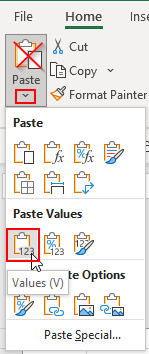
Use the ribbon: (1) Home (2) Paste and (3) Paste Special (as shown in the screenshot above).	Use one of the key combinations Alt E (for Paste) then S (for Special) or Ctrl Alt V (as shown in the screenshot above).

Either way, you are then presented with the paste special dialogue box which offers lots of options, which we will now review.
In each case, select the option(s) you want and click OK or press enter on your keyboard to complete the special paste.

 What Paste Special options do I have?

The Paste Special dialogue box is organised into three areas marked above, to answer these three questions:

1. What do you want to paste?
2. What operation should be carried out, if any?
3. What special actions should be performed, if any?

Within each area, you can only select one option. Combinations of options across areas are sometimes allowed, sometimes not, depending on what you have selected. Unavailable options are automatically greyed out by Excel.

So let’s look at these three areas in turn.

1. What do you want to paste?

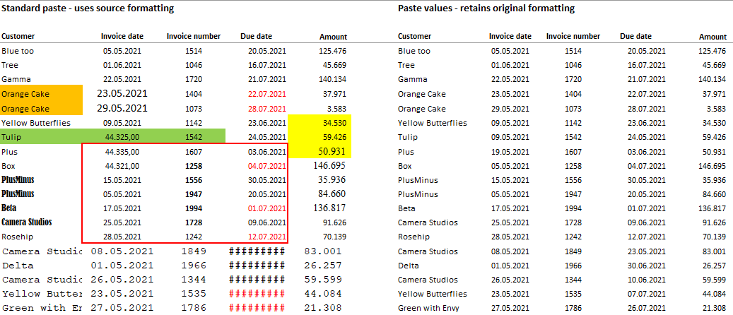
The default is “All”, which is the same as standard paste if no other options are selected. This means everything is pasted including formulas, font and background formats, comments and notes.

The options I use the most here are:

• Formulas - pastes formulas only and nothing else, so formats validations and borders remain unchanged in the pasted-to cells. Example use: copy a formula from a cell which is formatted bold to other cells which are not bold and which should remain so.
  
  
• Values - pastes values only and nothing else. This option is so useful, it has its own blog!
  
  
• Formats – pastes formats only and nothing else. Example use: copy the number formatting from a cell which is correctly formatted (such as a data cell) to other cells, some of which contain other formulas (such as SUM formulas).
  
  
• Validation – pastes validation rules only and nothing else. These are the rules you can set up using data, data validation e.g., to restrict inputs to only positive numbers (see my video on data validation for more details). Example use: copy the validation from some input cells requiring positive numbers and which also contain data to other input cells also requiring positive numbers but where the copied data would not be relevant.
  
  
• All except borders - pastes everything (including formulas, font and background formats) but not borders. Example use: copy a SUM formula from one column to other columns where the column at the end has a border which you want to keep.
  
  
• Column widths - pastes only the column widths and nothing else. Example use: you have multiple sheets which should have the same look and feel and want to ensure that the column widths are identical across the sheets.

 

2. What operation should be carried out, if any?

The default is “none”, which is usually what you want. But you can choose to add, subtract, multiply or divide. These actions are typically performed on inputs only, not on formulas. Example uses here include:

• Add or Subtract – Example use: In a sales planning, increase the planned number of units to be sold in each period by 100: Enter 100 in a cell and copy it, select destination cells and paste special, add.
  
  
• Multiply or Divide – Example use: Convert data in Euros to thousands of Euros: Enter 1000 in a cell and copy it, select destination cells and paste special, divide.
  
  

These can also be used to anonymise confidential data for training or demonstration purposes.

3. What special actions should be performed, if any?

These are the paste special specials and there are three on offer, the first two of which can be combined.

• Skip blanks – pastes only those copied cells with content and ignores any which are blank. Example use: in one workbook you have formulas to calculate actual sales values by brand (and no sub-totals or totals) and you want to paste these as values into an input area in a planning model but this has formulas for sub-totals and totals which you don't want to overwrite. Use the combination: paste special, values and skip blanks.
  
  
• Transpose – pastes copied content and switches it from horizontal to vertical or vice versa. Example use: you have monthly values arranged horizontally and want to paste them into an area where the months are arranged vertically, like this:
  
  
  
• Paste link – pastes a link to the copied cell(s). If you use this for one cell, the link is fixed for both column and row. Example use: You copy a key input cell (say the selected scenario or the master check result) and do a paste special, paste link to this cell in the main output sheet. The result is the same as the normal method of starting in the main output sheet and entering a formula = source cell. But paste link may be more efficient If you are already on the source sheet.
  
  

how2excel tips

1. Use the keyboard to quickly select options

In the Paste Special dialog box, all options have one letter underlined e.g. V in Values. Simply type this letter to activate the option. Finally press Enter on the keyboard to carry out your Paste Special.

2. Paste Special repeatedly

As with standard paste, you can paste special repeatedly, if necessary. This is possible as long as the copied data is still in memory, which is indicated by this message in the status bar at the bottom: of Excel.

Expert tip: Alternatively view the clipboard to manage all recently copied items and paste any of them.

That’s it! I hope you liked this special blog on paste special which I wrote specially for you!

Did you know you can easily paste copied data as values?

Why?

1) To keep your original formatting
If you do a standard paste (e.g. Ctrl V), everything gets pasted including formats - this includes font size and colour, background colour, and borders! Here you can compare a standard paste with a value paste - which do you prefer?

2) To avoid lots of “clutter”
Because a standard paste copies everything including cell protection, conditional formatting, and data validation, repeated use just clogs up your spreadsheet with unnecessary content. This can increase file size and can really hinder usage if you are using sheet protection.

3) To replace formulas with results (text or values)
This can be useful if you added some data to a table using a lookup formula but just want to keep the results as text or numbers.

How? Easy!

Mouse: Instead of just using standard paste (e.g. Paste button) click the down arrow to get options and then use the “paste values” button (clipboard icon with 123). Keyboard: Use Ctrl V, followed by Ctrl to get a drop-down list of options then V to select Values. (Thanks to Wyn Hopkins for that tip). Or you can use the 4-key sequence Alt H V V. Have fun with that!

Check out all the other ⚡ special paste options in our separate blog.

Create an interest and repayment plan for a loan yourself in Excel - we explain how! Or simply download our free Loan_Amortisation_Schedules with four plan versions, ready to use.

When do I need this?

If you need to plan an annuity or constant repayment loan (amortising loan) with regular (usually monthly) payments, perhaps as part of a financial model. Such a schedule can also be used to calculate liability values for finance leases / IFRS16. It can also be used to compare various financing alternatives with different terms and different interest rates.

Or maybe you just want to get a better understanding of that mortgage payment plan your bank is sending you. 😊

What is an amortising loan?

An amortising loan must be repaid (amortised) regularly over the term. There are two variants:

1. Equal instalments (annuity)

An annuity is a loan (or finance lease liability) where the instalments (interest and principal combined) remain constant throughout the term. Such loans are popular for both lenders and borrowers because the monthly cash flows are constant and predictable.

Each loan repayment includes some interest and some principal repayment which reduces the outstanding loan. Initially, the outstanding loan balance is at its highest and therefore the interest cost is also at its highest. As payments get made, the loan balance reduces gradually and consequently the amount of interest reduces so that more and more of the fixed monthly repayment goes towards repaying the loan.

2. Equal repayments

In the case of a loan with equal repayments, the amount of the regular payment to be made (interest and repayment together) decreases over time, because the repayment instalments remain the same but the interest on the remaining capital decreases.

How do I capture the basic loan details?

Create an input section for the basic data such as loan term etc., like this.

How do I calculate the monthly amounts?

Create a calculation section like this. Having the dates and amounts along the rows is standard practice in the financial industry. However, if using the calculations as an input for a financial model which is usually built across columns, it could make sense to build the loan schedule in columns as well. Just make sure you get the cell references correct.

You need a row for each period. In each period, you must calculate the interest, the principal, and the total instalment plus the closing balance. See below for details of calculation methods and formulas. A totals row at the top gives you a great overview and is ideal to check your results including the final closing balance (use an INDEX/MATCH function to find your closing balance).

To make things easy for you, we have created a file with four loan schedules which you can download free of charge: Loan_Amortisation_Schedules.

They also include visualisations to show how the payments and balances change over time.

 How can I use one of the loan schedules available in downloads?

You can use any one of them ‘as is’ by simply amending the assumptions (grey input cells at the top). Alternatively, you can incorporate one into an existing model. In this case, copy the relevant calculation into your model, then link the interest costs to your profit and loss account (income statement) and the closing balances to your balance sheet. For a cash planning tool, link the total installments as cash outflows to your cash flow plan.

What does each schedule do, exactly?

Each schedule automatically calculates your monthly instalments (split into interest and principal) and the remaining balance. Furthermore, it visually highlights the current period row in green based on today’s date.

In schedule 4 (fixed principal repayment) you can also enter one-off repayments as inputs right next to each period. The remaining principal repayments will automatically be adjusted.

There are four versions - what are the differences?

The four versions differ in the way the interest, principal repayment and the total instalment are calculated, as follows.

Vers.	Short description	Interest	+ Principal repayment	= Total instalment	Closing balance
1	Uses Excel financial functions	=IPMT(rate, per, nper, pv, [fv], [type])	=PPMT(rate, per, nper, pv, [fv], [type])	=Interest + Principal	=Closing bal. prior period - principal repayment
2	Mostly uses  mathematical operators	=Outstanding loan balance * annual interest rate/12	=Total instalment - Interest	=PMT(rate, nper, pv, [fv], [type = 0])	Same as version 1
3	Same as version 2, but payments in advance	First period is zero, otherwise same as version 2	Same as version 2	=PMT(rate, nper, pv, [fv], [type = 1]) plus balloon in final month	Same as version 1
4	Same as version 2, but with fixed principal repayments	Same as version 2	Equal  instalments reduced by any one-off repayments	=Interest + Principal	Same as version 1

 Notes

• Version 1: Excel functions do the hard work for you!
  Any balloon payment is shown as a remaining balance at the end of the term.
  
  
• Version 2: Some modellers are more comfortable with this approach and it is more flexible than version 1 e.g., if you need to model ad-hoc repayments.
  
  
• Versions 1 and 2: These are both based on payments in arrears and yield the same results. There are almost always various routes to success in Excel and this is a great example.
  
  
• Version 3: Covers the special case of lease contracts with payments in advance and a residual value guaranteed by the lessee at the end of the term (common structure in Germany). The guaranteed residual value/balloon payment is shown as being paid at the end of the last month of the term. It still accrues interest over that period.
  
  
• Version 4: Payments in arrears with a fixed principal repayment that changes only if additional one-off principal payments are made.
  Any balloon payment is shown as a payment at the end of the term.
  
  

In the Excel financial functions, what do ‘rate’, ‘per’ etc. mean? 

All three financial functions used (IPMT, PPMT and PMT) use the same arguments which are now explained. To help you, we added the relevant term next to each of the input cells.

• nper: The total number of payment periods for your annuity.
  
  
• per: The period number for which you want to find the interest or principal repayment. Must be in the range 1 to nper. (This figure is not in the assumptions but in the first column in the loan schedule, called ‘Period’).
  
  
• rate: The interest rate per period, usually the monthly or annual rate.
  
  
• pv: The present value (initial amount) of the loan or financial lease.
  
  
• fv (optional): The future value or balance after the last payment is made. If fv is omitted, it is assumed to be 0. The future value of a loan, for example, is typically 0.
  
  
• type (optional): Enter 0 for payments made at end of each period or 1 for payments made at the beginning of each period. If type is omitted, it is assumed to be 0.
  
  

Warning! Take care when using these functions that the rate, per and nper arguments match up i.e., if you are using monthly periods (as here), then the interest rate also has to be monthly not annual. If you mix them up you will get incorrect results!

Also, make sure you use the correct signs in the formula i.e., when pv is positive, fv needs to be negative and the other way around to get the correct values. If you use pv as a positive number, your formula results will be negative numbers (which you might have to convert depending on what you are planning to use them for).

Which version is best to use?

For standard loan structures (payment in arrears) you are free to choose your preferred version between versions 1 and 2. For leasing structures with payment in advance version 3 is your template of choice. For loans with equal principal repayments in each period (with or without additional / one-off  principal repayments), please use version 4.

What special features do the schedules have?

• Data validation for the terms input cell (D6): inputs must be a whole number between one and 360 in order for the formulas to work correctly.
  

How? Please select cell D6, use the menu Data , Data Validation, and review the ‘Settings’ and ‘Error Alert’ tabs

• Conditional formatting for the table: the data for the current month is automatically highlighted with a green background.

How? Please select any relevant cell, use the menu Home, Conditional Formatting, Manage Rules and review the settings

 

 

What do the motivation levels of the Excel pyramid mean for you and how can you climb them? In this blog I will answer both questions and give you links to useful resources.

In time-honoured tradition, we start at the bottom and work our way up through the levels. Before we start, there is one piece of valuable advice which is valid for all levels:

Constantly learn and grow your Excel skills and practice these as often as you can to make sure they become second nature. Or as I like to say at the end of my training courses: “use it or lose it!"

 

Physiological

You have a PC or laptop with MS Office installed, can open Excel and enter data and formulas

This level is easy to achieve. If you have a PC or laptop, you probably have MS Office already installed. Fire up Excel and you are ready to get cracking with data and calculations. Especially, but not only, for beginners I recommend the following great website.

https://www.excel-easy.com/

This has hundreds of practical examples organised in useful topics. Pick a topic area and work through the pages and examples to learn the topic. Alternatively, you can search the entire site using the search box at the upper right of the start page to find what you are looking for.

 

Safety

You develop your spreadsheets according to best-practice (e.g., clear inputs, no hard-coding) and include model checks to catch errors

Once you have the basics under your belt, it is important to learn best practice so that you do not develop bad habits such as hard-coding (entering a number in a formula rather than referring to an input cell with the value) and to help ensure that your spreadsheets are reliable.

For this you can follow

Gary's Golden Ground Rules

or the „20 Principles for Good Spreadsheet Practice“ from the Institute of Chartered Accountants of England and Wales (ICAEW).

https://www.icaew.com/technical/technology/excel-community/twenty-principles

 

Love/belonging

Users love using your spreadsheets because they have user-friendly design and great functionality

Cash may be king for financial models, but outputs are king for spreadsheets. What you need is clarity and impact. Where better to find out more than a website and book called “Clarity and impact” from Jon Moon.

https://www.jmoon.co.uk/

Among other things, you will learn the four principles of great design: contrast, repetition, alignment, and proximity which can also be applied to spreadsheets (and which just happen to have an easy-to-remember acronym!)

For great functionality, I suggest you learn tricks and tips. One useful website is the one you are currently on! To my knowledge, we are unique in offering all content in both English and German.

www.how2excel.com

I am a fan of the ExcelJet website, where I learned dynamic arrays. The site includes short training videos and you can also sign up for a useful newsletter.

https://exceljet.net/

If you like youtube, check out Leila Gharani’s channel which offers lots of great learning videos for Excel.

https://www.youtube.com/channel/UCJtUOos_MwJa_Ewii-R3cJA

 

Esteem

You are valued because your spreadsheets help users in their work

At the latest by this stage, you need to adopt a formal approach to developing your workbooks. The best way to learn here is with structured training courses which take you through a topic step by step, building up your knowledge and your skills as you go.

I am a big fan of Maven Analytics – their online courses are very professional and well-structured and often have useful additional material to download. These includes courses on Power Query and Power BI. You can buy their courses on Udemy. Never pay full price here - all courses are regularly on offer for around €14.99.

https://www.udemy.com/courses/search/?q=maven+analytics&src=sac&kw=maven+anal

If live training is more suitable for you or your organisation, my consulting business Knott Consulting offers that – either on-site or remote, in English or German. We offer a broad range of courses from data analysis and planning to intermediate and advanced business modelling, as well as customised courses e.g., for Power Query and VBA macros. Participants complete structured case studies with support from experienced and motivated trainers to maximise their learn effect. For more details, please visit our website

https://www.knott-consulting.com/en/excel-training/

 

Self-actualisation

You are an Excel wizard and know how to excel at any calculation

On your way to reaching this level you will need to learn to develop 3-way financial models, so called because they include three financial statements: profit and loss account (sometimes called income statement), balance sheet and cashflow, which all impact one another. A good start is the free course from Gridlines.

https://academy.gridlines.com/p/essential-financial-modelling

At Knott Consulting (see link above) we offer this as well as M&A modelling and discounted cash flows (DCF) as live training (on-site or remote). Alternatively, you can teach yourself M&A and DCF modelling e.g. at Macabacus.

https://macabacus.com/learn

You may choose to get professionally certified by either CFI or FMI:

https://corporatefinanceinstitute.com/collections/ (FMVA® certification)

https://fminstitute.com/ (3 levels: Advanced, Chartered and Master Financial Modeler)

The CFI certification includes course material. For FMI, you need to use an external trainer such as Danielle Stein Fairhurst. Her company Plum Solutions offers FMI exam preparation and a range of other training courses.

https://plumsolutions.com.au/

And finally, you can sign up to be a Full Stack Modeller. This covers a wide range of skills needed by Excel masters from soft skills like having the correct mindset through to the latest tools technology has to offer in modelling, data processing and analysis.

https://www.fullstackmodeller.com/

 

The path to the top

Those are not the only routes you can take. There are lots of other great sites and trainers out there, I have mentioned here those sites and people that have particularly inspired me or others I know or who I have learnt a lot from. Whatever path you take, get out there and learn and practice to climb the Excel pyramid.

I would like to close this blog by quoting words of wisdom from the great (Jedi) master himself, Yoda!

“Always pass on what you have learned.”

That way, others can benefit from your knowledge and skills – and that is the best reward of all! 😊

Filters are great for, well, filtering data so you only see rows of data which you are interested in, e.g., invoices for a certain customer. Here I show you three quick tips to help you in your daily work.

Tip 1: Use a shortcut to turn filters on

Select any cell in your header row or in the data and use the shortcut Ctrl Shift L to turn on the filters in the first row. If you add an extra column at the right of your data, this is not automatically added to the filter range. Use the shortcut twice to turn the old filters off and the new filters on to include the new column.

Tip 2: Avoid empty or incomplete filter lists

If a filter shows no data, or is missing items, this is because Excel did not correctly recognise the data range e.g., because you have  a blank row at the top of your data. In this case, you should manually select the complete data range that you wish to filter, then turn the filter on.

Tip 3: Quickly filter for #N/A values

If you want to filter for #N/A entries to investigate errors, the usual method is to deselect all items, then scroll down to the list and select the entry #N/A which is always at the end of the list. If the number of items is long, this can take a while.

A much quicker approach is to simply type # in the search box... and that's it!

A similar trick can be used to filter for blanks which are also shown at the end of the list. Here you can start to type the word (Blanks) into the search field - usually the opening bracket ( is sufficient to filter the list.

Your vote counts! It would be much easier if Excel would show the #N/As and (blanks) at the top of the filter list. Vote for this idea here.

Want more filter tips? Watch my short filter tips video.