Create an interest and repayment plan for a loan yourself in Excel - we explain how! Or simply download our free Loan_Amortisation_Schedules with four plan versions, ready to use.
When do I need this?
If you need to plan an annuity or constant repayment loan (amortising loan) with regular (usually monthly) payments, perhaps as part of a financial model. Such a schedule can also be used to calculate liability values for finance leases / IFRS16. It can also be used to compare various financing alternatives with different terms and different interest rates.
Or maybe you just want to get a better understanding of that mortgage payment plan your bank is sending you. 😊
What is an amortising loan?
An amortising loan must be repaid (amortised) regularly over the term. There are two variants:
1. Equal instalments (annuity)
An annuity is a loan (or finance lease liability) where the instalments (interest and principal combined) remain constant throughout the term. Such loans are popular for both lenders and borrowers because the monthly cash flows are constant and predictable.
Each loan repayment includes some interest and some principal repayment which reduces the outstanding loan. Initially, the outstanding loan balance is at its highest and therefore the interest cost is also at its highest. As payments get made, the loan balance reduces gradually and consequently the amount of interest reduces so that more and more of the fixed monthly repayment goes towards repaying the loan.
2. Equal repayments
In the case of a loan with equal repayments, the amount of the regular payment to be made (interest and repayment together) decreases over time, because the repayment instalments remain the same but the interest on the remaining capital decreases.
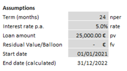
How do I capture the basic loan details?
Create an input section for the basic data such as loan term etc., like this.
How do I calculate the monthly amounts?
Create a calculation section like this. Having the dates and amounts along the rows is standard practice in the financial industry. However, if using the calculations as an input for a financial model which is usually built across columns, it could make sense to build the loan schedule in columns as well. Just make sure you get the cell references correct.
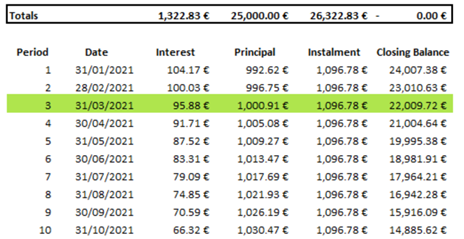
You need a row for each period. In each period, you must calculate the interest, the principal, and the total instalment plus the closing balance. See below for details of calculation methods and formulas. A totals row at the top gives you a great overview and is ideal to check your results including the final closing balance (use an INDEX/MATCH function to find your closing balance).
To make things easy for you, we have created a file with four loan schedules which you can download free of charge: Loan_Amortisation_Schedules.
They also include visualisations to show how the payments and balances change over time.
How can I use one of the loan schedules available in downloads?
You can use any one of them ‘as is’ by simply amending the assumptions (grey input cells at the top). Alternatively, you can incorporate one into an existing model. In this case, copy the relevant calculation into your model, then link the interest costs to your profit and loss account (income statement) and the closing balances to your balance sheet. For a cash planning tool, link the total installments as cash outflows to your cash flow plan.
What does each schedule do, exactly?
Each schedule automatically calculates your monthly instalments (split into interest and principal) and the remaining balance. Furthermore, it visually highlights the current period row in green based on today’s date.
In schedule 4 (fixed principal repayment) you can also enter one-off repayments as inputs right next to each period. The remaining principal repayments will automatically be adjusted.
There are four versions - what are the differences?
The four versions differ in the way the interest, principal repayment and the total instalment are calculated, as follows.
|
Vers. |
Short description |
Interest |
+ Principal |
= Total instalment |
Closing balance |
|
1 |
Uses Excel financial functions |
=IPMT(rate, per, nper, pv, [fv], [type]) |
=PPMT(rate, per, |
=Interest + Principal |
=Closing bal. |
|
2 |
Mostly uses mathematical operators |
=Outstanding loan balance * annual interest rate/12 |
=Total instalment |
=PMT(rate, nper, pv, [fv], |
Same as |
|
3 |
Same as version 2, but payments in advance |
First period is zero, otherwise same as version 2 |
Same as |
=PMT(rate, nper, pv, [fv], |
Same as |
|
4 |
Same as version 2, but with fixed principal repayments |
Same as |
Equal instalments reduced by any one-off repayments |
=Interest + Principal |
Same as |
Notes
- Version 1: Excel functions do the hard work for you!
Any balloon payment is shown as a remaining balance at the end of the term.
- Version 2: Some modellers are more comfortable with this approach and it is more flexible than version 1 e.g., if you need to model ad-hoc repayments.
- Versions 1 and 2: These are both based on payments in arrears and yield the same results. There are almost always various routes to success in Excel and this is a great example.
- Version 3: Covers the special case of lease contracts with payments in advance and a residual value guaranteed by the lessee at the end of the term (common structure in Germany). The guaranteed residual value/balloon payment is shown as being paid at the end of the last month of the term. It still accrues interest over that period.
- Version 4: Payments in arrears with a fixed principal repayment that changes only if additional one-off principal payments are made.
Any balloon payment is shown as a payment at the end of the term.
In the Excel financial functions, what do ‘rate’, ‘per’ etc. mean?
All three financial functions used (IPMT, PPMT and PMT) use the same arguments which are now explained. To help you, we added the relevant term next to each of the input cells.
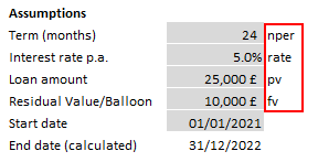
- nper: The total number of payment periods for your annuity.
- per: The period number for which you want to find the interest or principal repayment. Must be in the range 1 to nper. (This figure is not in the assumptions but in the first column in the loan schedule, called ‘Period’).
- rate: The interest rate per period, usually the monthly or annual rate.
- pv: The present value (initial amount) of the loan or financial lease.
- fv (optional): The future value or balance after the last payment is made. If fv is omitted, it is assumed to be 0. The future value of a loan, for example, is typically 0.
- type (optional): Enter 0 for payments made at end of each period or 1 for payments made at the beginning of each period. If type is omitted, it is assumed to be 0.
Warning! Take care when using these functions that the rate, per and nper arguments match up i.e., if you are using monthly periods (as here), then the interest rate also has to be monthly not annual. If you mix them up you will get incorrect results!
Also, make sure you use the correct signs in the formula i.e., when pv is positive, fv needs to be negative and the other way around to get the correct values. If you use pv as a positive number, your formula results will be negative numbers (which you might have to convert depending on what you are planning to use them for).
Which version is best to use?
For standard loan structures (payment in arrears) you are free to choose your preferred version between versions 1 and 2. For leasing structures with payment in advance version 3 is your template of choice. For loans with equal principal repayments in each period (with or without additional / one-off principal repayments), please use version 4.
What special features do the schedules have?
- Data validation for the terms input cell (D6): inputs must be a whole number between one and 360 in order for the formulas to work correctly.
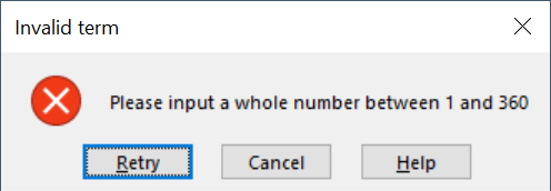
How? Please select cell D6, use the menu Data , Data Validation, and review the ‘Settings’ and ‘Error Alert’ tabs
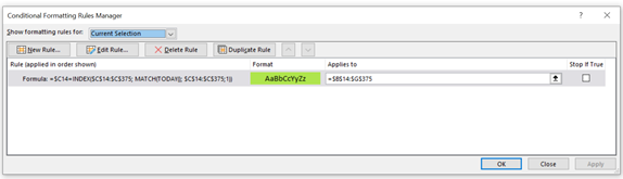
- Conditional formatting for the table: the data for the current month is automatically highlighted with a green background.
![]()
How? Please select any relevant cell, use the menu Home, Conditional Formatting, Manage Rules and review the settings