
Filters are great for, well, filtering data so you only see rows of data which you are interested in, e.g., invoices for a certain customer. Here I show you three quick tips to help you in your daily work.
Tip 1: Use a shortcut to turn filters on
Select any cell in your header row or in the data and use the shortcut Ctrl Shift L to turn on the filters in the first row. If you add an extra column at the right of your data, this is not automatically added to the filter range. Use the shortcut twice to turn the old filters off and the new filters on to include the new column.
Tip 2: Avoid empty or incomplete filter lists
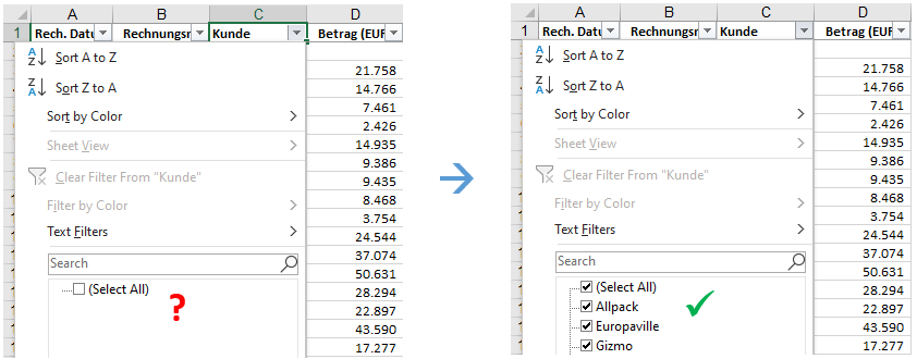
If a filter shows no data, or is missing items, this is because Excel did not correctly recognise the data range e.g., because you have a blank row at the top of your data. In this case, you should manually select the complete data range that you wish to filter, then turn the filter on.
Tip 3: Quickly filter for #N/A values
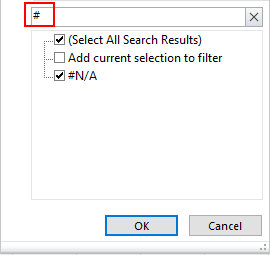
If you want to filter for #N/A entries to investigate errors, the usual method is to deselect all items, then scroll down to the list and select the entry #N/A which is always at the end of the list. If the number of items is long, this can take a while.
A much quicker approach is to simply type # in the search box... and that's it!
A similar trick can be used to filter for blanks which are also shown at the end of the list. Here you can start to type the word (Blanks) into the search field - usually the opening bracket ( is sufficient to filter the list.
Your vote counts! It would be much easier if Excel would show the #N/As and (blanks) at the top of the filter list. Vote for this idea here.
Want more filter tips? Watch my short filter tips video.