Category: Blog EN

But surely you need to use both?

Yes and no… some tasks can only (efficiently) be performed by one or the other. For example, data entry: a keyboard is the obvious tool of choice. But you may be surprised at how many tasks can be completed be either. Typically, we are talking here about marking and amending blocks of data, inserting rows or columns, copy and pasting etc. All tasks commonly performed when working in Excel.

Why does it matter?

You may be surprised how much more efficiently you can work with the appropriate tool. Spoiler alert… at this stage I can reveal that I am a big fan of keyboard shortcuts which can dramatically reduce the time needed to perform especially simple tasks like copy and paste. Added up over the course of a working day, these small savings of time add up and can result in you simply being able to get more work done! And all for a little effort required in learning to use shortcuts.

What do you mean “best to use”?

Before we dive in, let’s be clear about what we mean by “best to use”. It is the user that uses these tools, so we need to consider him or her… therefore I would define this to mean most appropriate and most efficient for the user.

What are the options?

To make my analysis comprehensive, I have considered two types of mouse – the mousepad you usually get with a laptop nowadays and a separate, “old school” mouse – as well as two types of keyboard – again, the one you get with a laptop and a separate keyboard, the type you have to use if you are using a desktop PC and which is optional when using a laptop.

Tool	😊 Advantages	☹ Disadvantages
Laptop mousepad	Can be used on a plane or train, where the table is small and there is no room to use a separate mouse Hard to forget… if you have your laptop with you on a business trip, then you also have your mouse!	I find them extremely inefficient to use; to move the mouse pointer any length over the screen requires multiple touchpad strokes; only experienced users can hope to come anywhere near the efficiency of the other tools For non-users, must be turned off to avoid “ghost working” (accidental activity caused be inadvertently touching the touchpad)
Separate mouse	Generally, much more efficient than the laptop mouse Enables menus and icons to be easily used Particularly good for inexperienced users – easy to use and no need to remember keyboard shortcuts	Often not as efficient as keyboard shortcuts for frequent tasks such as copy & paste (Ctrl C, Ctrl V) Usage requires more space on your desk or work surface
Laptop keyboard	Compact – does not take up much space You can use the full gamut of keyboard shortcuts, albeit this can be somewhat awkward (see disadvantages) No need to research and buy a separate keyboard	Compact, so functions are often combined into single keys, thus requiring laborious (dare I say tortuous?) key combinations to get what you want, e.g. using the function keys such as F2 edit where you often have to press a “function-enabling key” as well as the function key itself… yuk! No separate number keypad to enter numbers, which I tend to do a lot in Excel!
Separate keyboard	You can use the full gamut of keyboard shortcuts… yahoo! A real boon to all who know them or learn some of them! You usually get a separate number keypad to enter numbers; a common task when using Excel Function keys can usually be operated on their own without the need to press any “function-enabling key” (sadly not always the case)	Tasks up space on the desk; IMHO this is more offset by the advantages More space means more keys and sadly a higher risk of additional keys with functions which I never use and/or which do not always work (media start/stop, home, arrange Windows, settings, picture etc) I am such a fan, I will sometimes take my separate keyboard to meetings where I expect to have to do a lot of computer work; this is then something extra to transport

To sum up, many common tasks in Excel can be performed by either mouse or keyboard, so you have a choice. I recommend the keyboard – ideally a standalone keyboard - so that you can use time-saving shortcuts. You can download a list of the best shortcuts under downloads.

https://www.how2excel.com/en/downloads-2/

This is A4 in size, but you can fold it in half in the middle to have A5 size with two sides if that suits you better. The best way to learn these is "little and often". Pick one or two new shortcuts each week and use them as often as you can to make them second nature. Some people like to use a highlighter pen to mark the ones they have learnt to show progress and aid motivation.

Have fun!

I hope you are also a fan of SUMIFS… this great function can be extremely useful for adding up sub-sets of data. But it has two limitations:

1. Performing calculations on data in other files is not best practice, but it can be a practical solution in some cases. In such cases, a SUMIFS formula can generate errors if the other file is closed.
2. You cannot have criteria in two dimensions (rows AND columns), just one or the other.

There is a way to solve both these issues using the function SUMPRODUCT.

1. SUMPRODUCT in one dimension

Here is an example using small table of data.

As you can see, the formula is like the equivalent SUMIFS formula. Here, however, each criteria range is not separated from its related criteria by a separator (typically a comma or semicolon, depending on your regional settings). Instead, they are separated by an equals sign, which I find easier to read. Each (criteria range = criteria) test is surrounded by brackets and multiplied with the next (criteria range = criteria) test. At the end, you must multiply by one to convert all the true and false results into 1s and 0s and lastly you multiply by the data range which is to be summed. With SUMIF (1 criterion), this data range must be the first argument in the brackets, with SUMIFS (1+ criteria), it must be the last. With SUMPRODUCT, it can be either first or last.

External files

All the function arguments (the bits in the brackets) can refer to an external file.

how2tip: I find it easier to write and test such a formula in the file with the source data and then cut and paste it to the desired location. This is easier because you can (a) better see what you are referring to and (b) the path and file name do not appear in the formula until you cut and paste it, so it is easier to write, understand and test.

2. SUMPRODUCT in two dimensions

The above principles can now be extended to two dimensions, as shown here, using the same data table.

Here it is important that (similar to the one dimension example) the criteria ranges match the height or width of the data table, as you can see in the F2 (“edit mode”) screenshot above.

3. Conditional formatting

To put the icing on the cake, I decided to use conditional formatting to automatically highlight (in green) the data cells being added up. These vary, depending upon what criteria are selected in the salmon-coloured input cells.

The conditional format must be applied to the all data cells in the table since any of them could fulfil the selected conditions.

The format must highlight cells (in this case in green) if all conditions in the SUMPRODUCT formula are fulfilled, as shown below. Here it is important to pay attention to the dollar (fixing) symbols. Always write the formula from the viewpoint of the cell in the upper left corner of the data range, here C3. The formula must start with an equals sign (as in all Excel formulas) und must give a true or false result. It is the equivalent of writing an IF formula, but you do not need the IF function. Just write the logical test, using “OR” or “AND” as required.

That’s it, have fun!

You can work more efficiently in Excel if you can navigate effectively. With regular practice of the methods I explain below, you too can become an expert in Excel navigation!

Navigation in and around Excel can be divided into three main task areas. You can perform all three types of task with the mouse, but using the keyboard is usually more efficient, largely because you need to perform less steps than with the mouse.

1. Navigate between open applications / documents

• Alt + Tab --> cycle between all open applications / documents

• Windows key + Tab --> shows all open applications / documents. Select one with the mouse or use the arrow keys to highlight the desired application / document and then press enter to select it

• Ctrl + Tab (in Excel) --> cycle between all open workbooks
   

2. Navigate between worksheets

• Ctrl + Page Up or Down --> move from one worksheet to the next

• (Mouse) Use the arrow buttons in the lower left corner of Excel  to shift the worksheet tabs in view; Press Ctrl at the same time to show the first or last worksheets

• Right-click on these arrow buttons to get a list of all worksheets in the model, click to jump

• If you have my toolKCit installed, use the button “List all sheet names” to create a new sheet with easy-to-use hypertext links
  
  Tip: my toolKCit contains this and 18 other useful tools - buy it at eloquens and use the discount code HOW2EXCEL to get 50% off

• Use range names:
  • Define: select cell(s) then type a range name, without blanks, in the name box below the toolbar e.g.
    
  • Use: Click on the name box down arrow, click on a name to jump there
     

3. Navigate within a worksheet

• Ctrl + Home --> select “home cell”

• Ctrl + End --> select “end cell”; if this is wrong i.e. includes many blank rows or columns then delete these and save the file to reduce the file size and possibly improve the calculation speed

• Alt + Page Up or Down --> move left or right, a screen at a time

• Use the arrow keys

Arrow key alone	With Ctrl	With Shift	With Ctrl + Shift
Move to the next cell	Move to the end of a cell block or to the next non-empty cell	Move and mark cells	Move in a block and also mark the cell range

• Ctrl + A or Ctrl + * --> select a complete block of cells

• You can also use many of these tips in Word
   

Have fun navigating!

PS. You can download this blog as a handy PDF here
Navigate_efficiently_in_Excel

Excel offers a huge variety of charts (also commonly called graphs) so it can be difficult to identify the most suitable type for presenting your data. Here I explain some basic guidelines which should help you pick the best type in several typical cases and some useful tips. I also give some advice on which chart types are not recommended.

What’s on offer?

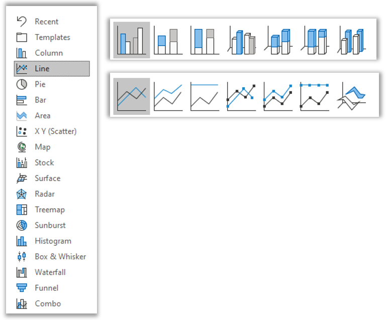
At the time of writing, Excel 365 offers 17 different chart types, shown below. Each type has several sub-types, shown below for column (bar chart) and line chart. You can also mix and match different types in a single chart, now called “Combo”. That means a lot of choice.

Does Excel offer any help?

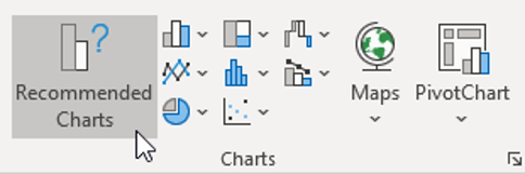
Yes - when you select data and move to Insert, Charts, Excel offers some recommended charts which you can review.

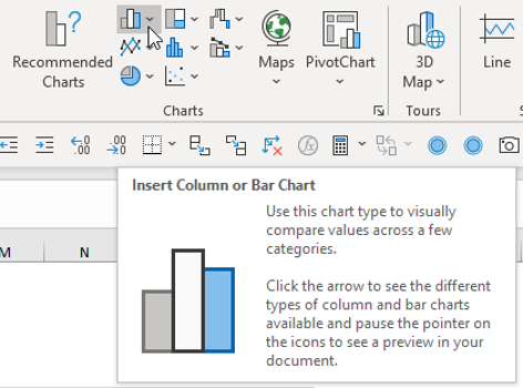
If you hover over a chart icon, Excel shows you a large tip box with guidance.

I don’t always agree with the recommended chart types or the tips given, however, so I prefer to select my own using the following principles.

What type of data do you have?

I have reviewed the charts in numerous spreadsheets and found that in over 90% of cases these fall into one of the following three categories, so I will focus on these.

1. Data over time
2. Data per category
3. Change in a single value over time or between e.g. plan and actual

1. Data over time

E.g. Sales per year or number of kilometres travelled per month

--> In this case I recommend a line chart as it is easier to see trends over time.

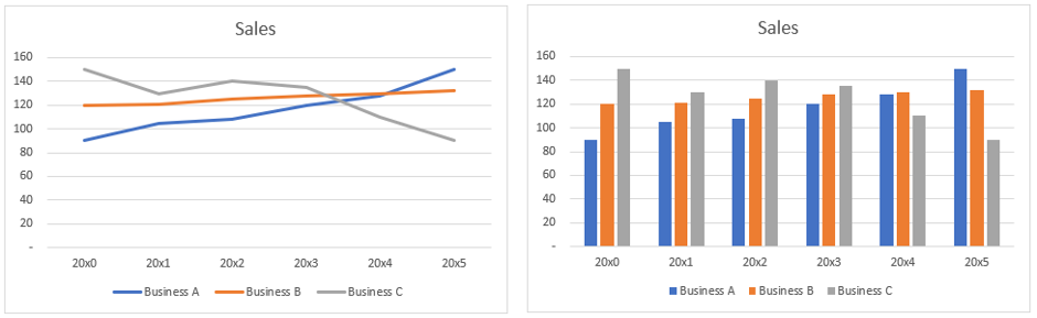
In the two charts above I have plotted the same data as both a line chart and a clustered bar chart. The line chart shows more clearly show that business A is a rising star, B is plodding along, and C is a falling star. In the clustered bar chart, this development is more difficult to see. In my opinion, this is more important than comparing businesses within each year, which is what the clustered bar chart enables you to do.

2. Data per category

E.g. number of customers per region or average amount spent in a month on various leisure time activities (such as going to the cinema) in different countries.

--> In this case I recommend a clustered or stacked bar chart to facilitate comparisons. There are several options, which I now compare.

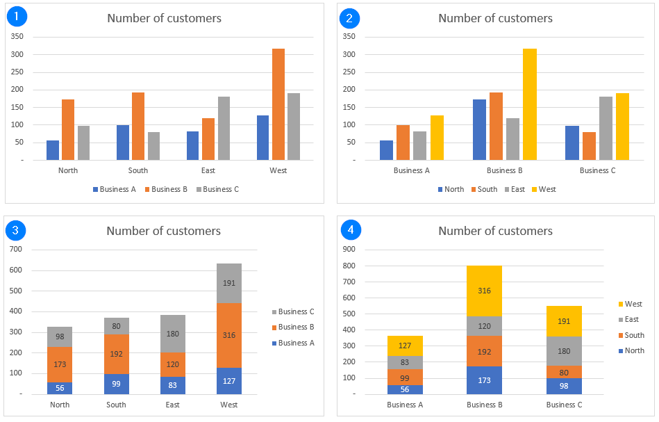
In the four charts above I have plotted the same data as clustered charts (1 and 2) and as stacked bar charts (3 and 4).

• Charts 1 and 3 are better to analyse the regions:
  (1) Here you can compare the businesses within each region
  (3) Here you can better compare regions against each other

• Charts 2 and 4 are better to analyse the businesses:
  (2) Here you can compare the regions within each business
  (4) Here you can better compare businesses against each other

• Ask yourself which chart version best presents the data for the analysis you are performing.
   

How2tips:

• In charts 3 and 4, I have added data labels as it is no longer easy to judge the size of each bar component; to do this, right-click on a coloured bar and select “Add data labels”; repeat for all other colours. Light coloured labels are better on dark backgrounds and vice-versa. To format labels, simply left-click on a label to select the series and then use the usual text formatting icons in the Home ribbon or right-click on a label and select format data labels.
   
• In charts 3 and 4, I have also moved the legend to the right-hand side. This matches the construction of the bars (e.g. in chart 4, from North at the bottom to West at the top) and so makes it easier to read what each colour in the bar represents. To do this, right-click on the legend, select "format legend" and then select legend position "right".
   
• In charts 1 and 2, it is better to have the legend at the bottom for similar reasons.
   
• You can change the chart type by right-clicking on the chart and selecting the aptly named “Change chart type.”
   

If some of your data is not split into discrete categories such as business regions but can instead take a wide range of values such as price or age, then you display your data grouped into clusters in a histogram. Examples here could be total sales of wine in different price categories or ice cream consumption per age group. A histogram is similar to a bar chart but each bar represents a given range of values such as wine priced up to €5 per bottle, €5 to €10 per bottle etc.

3. Change in a single value over time or between e.g. plan and actual

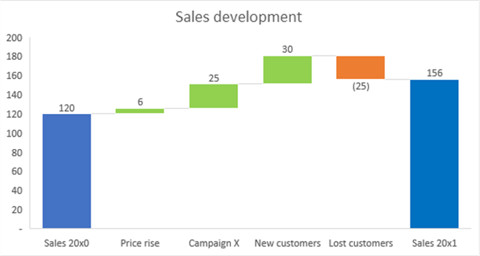
If you want to show how a certain value (typically sales or profit) changed from one year to the next, you can use a waterfall chart to show the changes, as shown above. This chart type is only available as standard from Excel 2016. In older versions, you must create it yourself using stacked bar charts, with some bars having no colour.

Assuming you have Excel 2016 or later…

1. Set up your data with the starting and end values and the changes between them with a suitable short description in each case.
2. Select your data, then go to Insert, Charts, Waterfall
3. Select the first bar by clicking it (so only the first bar is selected) and in the "Format data point” dialog that appears select “Set as total”
4. Repeat for the final bar
5. Optionally select and change the colour of other bars if you don’t like the defaults

Conclusion: This chart type can be very useful, but it is not as flexible as other chart types e.g., changing the colours is not easy.

More details: see Microsoft or xelplus (Leila Gharani)

What if I have other data types or the line and bar charts don’t help me to tell my story?

• Here you should think about what you want to convey and try out different chart types to see which best does the job.
   

How2tips:

• If you are not convinced with one chart type, you can change the chart type, as noted above.
   
• Alternatively, you can copy and paste the chart and change the chart type of the second version so that you can compare chart types side by side. I did this for the four bar chart examples above.
   
• Please remember that a simple table may be clearer than a chart, especially an overloaded or unusual chart.
   

Are any chart types not to be recommended?

• Pie charts – this chart type is well loved but the data can always be presented in a better way, perhaps as a simple statement or table. For example, if you have 60% of people are in favour of X and 40% are against, this simple statement is all you need; a pie chart does not improve understanding.
   
• 3D – these often make it hard to read the values and the 3D effects distract from the data, which, presented in the best way, should speak for itself without gimmicks.

You have probably experienced it… you open an Excel file and get a message that the file is linked to one or more external sources.

If this was not expected, it could be that the file contains unintentional links which you may wish to review and remove. This is not always an easy task as there are at least six ways an Excel file can be linked to another source and not all of them allow easy removal. Let’s go through them in turn.

1. Formulas

   This is the easiest one to find and fix. Go to Data, Edit links… there you can see the files linked to and if the links are simply in formulas, you can click on “break links” to replace the formulas with values.

   

   Warning: You may not want to replace formulas with values. E.g. you copied a formula from another version of the file, and this was linked to a sheet called “inputs”. The copied formula in the new file is linked to the sheet “inputs” in the old file. What you really want is for the formula to link to the sheet called “inputs” in the current file. You can search for the file name (in this example “Source file”) in the spreadsheet, then review and amend the formulas found to remove the superfluous path and file name of the old file.

   If the formulas are not simple links to single cells in the source file but are more complex e.g. using SUMIFS then “break links” doesn’t always work. It also doesn’t work if one or more of the other linkage types exist, so I cover these below.

2. Range names 

   These are also easy to find. Go to Formulas, Name Manager.

   

   There you can see if any range names refer to cells in other spreadsheets and edit or delete them accordingly. If necessary, search for the range name in the spreadsheet to find where it is used and amend or replace the range name as appropriate.

   Other linkages can arise if you copy content from another spreadsheet. The content stays linked to the data in the original spreadsheet… a link to an external file.

3. Chart data
4. Pivot table data
5. Conditional formats
6. Data validation
7. Objects e.g.
   (i) a shape containing text linked to a cell
   (ii) a data slicer for a pivot table or a table
   (iii) a VBA control such as a button linked to a macro

These can be tricky to find, so try to work smarter not harder. What have you copied or otherwise changed in the spreadsheet since you opened it last time and didn’t get a message that the file was linked to one or more external sources? Then this is likely to be the cause of the link and can make it easier to find. Review those elements and you can maybe find and amend / remove the link as appropriate.

If that doesn’t help you, then you can find and review each element (e.g. each graph) in turn. Charts and pivot tables are easy to identify. You can find conditional formats and data validation using F5 (goto), special, then select conditional formats or data validation and OK.

The relevant cells on the selected sheet are then marked, and you can review them: Home, Conditional Formatting, Manage Rules or Data, Data Validation. Repeat for other sheets.

The brute force method

If that fails, and your spreadsheet is large then a brute force method may be the only way to identify the links. Very important: Make a back-up copy of your spreadsheet file for safety. Also make a copy of it to work on. You will have to partially destroy this file, so it is important to work on a copy only. In the copy file, start by selecting one or more sheets and either move them to a new workbook or alternatively delete them: right-click on a tab name and select 'Move or copy' or 'Delete'. Then save the file. See if the links remain. Sometimes it is necessary to close and reopen the file to force Excel to review the links.

• If the links are gone, they were in one or more of the sheets you moved or deleted. Move some sheets back into the main file or make another copy of the original Excel file and repeat the process, but delete fewer sheets. Do this until you have identified the offending sheet.
• If the links are not gone, move or delete more sheets then save and if necessary close and open the file until you identify the offending sheet.

 
Now you know a sheet with one or more links. You can then review the graphs, pivot tables, conditional formatting and data validation on this sheet. If the sheet is very large, you may need to move or delete sections of it (like the sheets move/deletion approach above) to narrow down where the external links are.

Once you find the link, open the original file and amend or remove the link there. Then save, close and reopen the file. If Excel still reports that there are external links, you will have to repeat the above steps in a new copy of the original file until you find and amend or remove all the links in the original file.

Good hunting!