Work faster with dynamic arrays

Excel's traditional approach requires us to use an array formula or rely on complex combinations of functions to achieve tasks like extracting unique values, sorting data, or filtering results.

But now dynamic array functions are here to simplify our lives and elevate our data analysis. 

In this blog I explain three of the key dynamic array functions: UNIQUE, SORT, and FILTER and give an example how these can be combined for stunningly effective results.


UNIQUE - Extracts unique items from a range of cells

Imagine you have a large dataset containing duplicate values. Previously, extracting unique values required convoluted formulas or manual effort. With the UNIQUE function, this process becomes effortless and instantaneous.

Suppose you have a list of sales data entries for various regions with duplicate entries. To extract the unique regions, you'd simply use the formula:

The UNIQUE function automatically returns a list of distinct values, saving you time and reducing the chance of errors.


SORT - Sorts a range of cells by a specified column

Sorting data in Excel is a routine task, but it can be cumbersome, especially when dealing with ever-changing datasets. Enter the SORT function, which brings a new level of simplicity and agility to the process.

Consider the above list of regions. To sort this data alphabetically, you'd use:

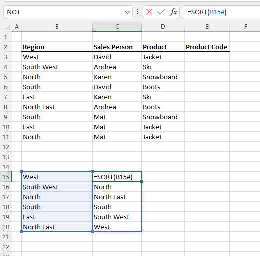
This function not only sorts your data but does so dynamically, adapting to new entries without requiring manual adjustments. Say goodbye to repeatedly re-sorting your data as it evolves.


Combination of SORT & UNIQUE

Combining SORT and UNIQUE will combine two steps into one and will always spill out the needed information as soon as data sets change.

The combination for the above data set will look as follows:

Always ensure you have enough free lines below your array / formula result as when data changes results can change.


FILTER - Filters data based in the criteria you define

Filtering data based on specific criteria often involves complex formulas and maintaining intricate cell ranges. The FILTER function turns this ordeal into a breeze.

Suppose you have the above sales table and want to see the data always broken up by your defined regions. To filter like this your formula and data can look like the below:

Now you can easily copy and paste the block of information and just change the region name (highlighted in yellow) –


With the FILTER function, you get an instantly updated result as your data changes, without the need to modify your formula. This feature is a game-changer for tracking dynamic trends and making data-driven decisions.


Advantages of dynamic arrays

Time Savings:

Dynamic array functions eliminate the need for complex array formulas or manual updates. What once took multiple formulas and adjustments now happens automatically, freeing up your time for more valuable tasks.

Accuracy:

With less room for manual error, your data manipulation becomes more reliable. The dynamic nature of these functions ensures that your results remain precise, even as your dataset evolves.

Flexibility:

Adaptability is key in today's data-driven landscape. Dynamic array functions seamlessly accommodate changes in data size, eliminating the need to constantly adjust formulas.

All of the above especially count when your data is arranged in a data table format.

Prevent user errors using data validation

I’m a big fan! To set this up, first select the relevant input cell(s) and mark these clearly with a consistent colour – perhaps using a predefined cell style - so the user can immediately see that the cell is for an input or a drop-down list (restricted list of inputs).

Click on the Data Validation icon in the Data ribbon under Data Tools. You get a dialog box with three tabs: Settings, Input Message and Error Alert. You must complete the Settings tab, the other two tabs are optional but also useful.


Settings

Firstly, you must decide what to allow under “Allow”. As a default, this is ‘Any value’. Select an option and complete the additional input fields, which then appear, to restrict the inputs which are allowed and click OK.

Here are the main options that I use with some example use screenshots, after the relevant validation rule has been set up.

  • Whole number
    Only integers from 1 to 5, e.g., for fixed asset useful lives in years or 1 to 12 for month.


  • Decimal (values that may have digits after the decimal point)
    For example, only decimals with positive values (greater than or equal to zero) for sales prices or only negative values for planned cash outflows for rent or tax payments.


  • List
    Probably my favourite! Allows you to allow only entries from a list. Either enter the list in the dialog box itself e.g., yes,no (with separators – either commas or semi-colons depending on your regional settings – but no spaces between list items) or link to a list in the model e.g., scenario names or cost centre numbers. Now when a user clicks in one of the restricted cells, they see a drop-down arrow which enables them to select a predefined item from the list.


  • Text length
    Good for product codes or postcodes which have a fixed length.

  • Custom
    Another of my favourites because it is extremely flexible. A formula is required: this must start with an equals sign and be followed by a test which gives a true or false result, i.e. what you would typically type when using an IF formula.

    For example, to ensure the data entered is a Monday enter this formula =WEEKDAY(C2,1)=2 where C2 is the cell with the data validation. Use $ fixing here, if appropriate. The formula can be tricky to get right so I recommend entering it as a normal formula in an Excel cell to test it. Once you are happy, you can copy the formula as text into the Data Validation, Custom, Formula field.


Input Message and Error Alert

You can also complete one or both of these optional tabs to advise users what type or range of data they must enter or why their input was not accepted - see screenshots above. This is useful because otherwise, if they input invalid data, they just get a standard error message with no clue as to what is wrong and what is acceptable.

On the ‘Error alert’ tab you can also decide what happens if input data does not meet the validation criteria. The default option is ‘stop’. Alternatively you can change this to a ‘warning’ or ‘information’. 

  • Stop: the default option - the data is not accepted.
  • Warning:  the user gets warned but can still go ahead – I use this for entries where I normally expect a negative value e.g., for a payment of taxes but which could, under certain circumstances be a positive value e.g., a tax refund.
  • Information: invalid entries are always allowed - this makes little sense in my opinion.


Learn more

  • Please see my video for more details and examples of how to set up data validation.
  • Data validation is just one of my top 6 tips to prevent user errors. Read my blog for the full list, which you can download as a PDF.

Size matters!

Look at the example shown below, which shows the same profit and loss statement first of all in whole Euros and then again in thousands of Euros (TEUR). Which column is easier to understand?

🏅 The second column wins hands down. This is because the average number of digits shown per number (significant figures) in the Euros column is 6 or 7 and in the TEUR column it is just 3 or 4, which is much easier to read and comparing columns (e.g. years) also becomes much easier.


Select appropriate units

Decide at the planning and design stage which units you will use for values in your workbook. The best units to choose depends upon the size of the numbers which you will be dealing with: the larger the numbers, the less digits you should show. For monetary units, I generally recommend either:

  • Thousands of Dollars/Pounds/Euros/etc. (with no decimal places) or
  • Millions of Dollars/Pounds/Euros/etc. (with one decimal place)

Select the units so that values shown have no more than 4 significant figures (visible digits in each number). This makes them easier to enter, use and interpret. Using too many digits not only make these tasks harder, but also gives a false sense of accuracy in plan figures.


State your units

Clearly state the units you are using at the top of each worksheet or even each row of your workbook, so users know what they represent.

You may wish to use whole dollars/pounds/euros in some circumstances, where this is more understandable and user-friendly – e.g. for price per article or average salary – but especially here you must clearly state the units. Ensure you convert results to the standard workbook units of (says) thousands of Euros for further calculations or outputs.

Compare workbooks

It can be very useful to compare two versions of the same workbook to see what has changed. Here are some tips to help you do just that.

  1. Open both files
    Open the old and new version of the workbook and select the same sheet. If you know where to look e.g., the assumptions sheet, select that sheet. Otherwise select an output sheet such as the financial statements.

  2. Check workbook settings

    If you have scenarios or other settings that affect outputs, ensure both versions have the same settings, so you are comparing apples with apples.

  3. Make them look the same

    Make sure the selected sheet in both workbooks is the same size e.g., 100% or 85%. You can find and change this in the lower right-hand corner. Ensure you have the same view in both e.g., by using the shortcut Ctrl Home/Pos1 to make sure the selected cell is the same in each workbook.

  4. Then make them look different

    So you can easily tell which workbook you are looking at, and also to avoid making changes in the old version by mistake, change the colour scheme in the old workbook under Page Layout, Colors, select color scheme – I find the garish “Red Orange” great for this purpose.

  5. Flick between the two workbooks
    Simply use the shortcut Ctrl Tab as often as you want. The human eye is very quick to identify changes so you can quickly identify what has changed. If necessary, do a single page down (shortcut Ctrl Pagedown) or page across (shortcut Alt Pagedown) in both workbooks to view and compare the next section.

  6. Alternatively, create a difference sheet

    Copy the sheet you are comparing and in the copied sheet, in the first cell with a number (e.g. D8), enter a comparison formula e.g.,
    ='Fin stats'!D8-'[2023-02-08 ProCam model v2.xlsx]Fin stats'!D8
    Then copy this to all relevant cells to see the changes.
    (Note: when you link to a single cell in another file, Excel fixes the cell referred to with $ symbols, please remove these before copying the formula).

  7. Drill-down
    Once you have found a difference and want to understand what is causing it (assuming it is not an input), trace one or more precedents in both workbooks and compare these using step 5 or 6.

    To trace precedents, use the Formulas ribbon, Formulas Auditing, Trace Precedents tool or use my all-time top tip: double-click to jump to the first precedent. For this to work, please check your settings: File, Options, Advanced, Editing options (first section), “Allow editing directly in cells” must be switched off (remove tick mark). See my video for details.

Tool tip: Microsoft also offers an Inquire tool that can compare workbooks for you, but unfortunately it is not available in all versions of Excel. Here are details from Microsoft on how to find out if you have it and how to use it, if you do.

Prevent Excel user errors

Here are my six top tips. You can download them as a useful checklist.

  1. Ensure users know which file to use (version control)

Before

After

  • Name files clearly including date or version number.
  • Move old files to sub-folders so that the main folder contains only the final version e.g., move prior versions sent out or used in meetings to “Archive” and back-ups to “zzz old”
  • Bonus tip: save space! In Windows explorer search for “zzz old”. Any folders that are older than (say) 6 months can be deleted as content is unlikely to be needed.


  1. Restrict access to authorised users only
  • Save files in server location with restricted access e.g., only finance department.
  • Add password to open or change, if appropriate: File, Save As, More options (under file name and type), Tools (next to Save button), General options…


  1. Develop workbooks using best practice rules for clarity and ease of use
  • Add a cover sheet showing contact person, workbook status and purpose, a list of sheets with short descriptions --> so users get a good overview and know who to contact in case of questions.
  • Use a clear workbook structure with separate sections for inputs, calculations, and outputs --> so users can understand the structure and easily find their way around.
  • Add an instructions sheet --> so users know how to use the workbook.
  • See my separate blog on 'Gary's Golden Ground-Rules' for details.


  1. Clearly mark input cells so users know what they may change
  • Use consistent formatting e.g., light grey with white border, protection turned off.
  • Define and use cell styles (on the Home ribbon) for ease of use.
    - Define: Click the drop-down arrow at the lower right and select "'New Cell Style' to define.
    - Use: Select cells to be formatted, then click on the relevant cell style in the ribbon.

Bonus tip: If you didn’t format your input cells as you created them, you can easily do that later. Here’s how to find and select all input cells on a sheet, to format them using your input cell style.

  • Select all cells using the mouse or shortcut Ctrl A (select all).
  • Press F5 --> the “Go To” dialogue box appears.
  • Click “Special…”, Constants and ensure only “Numbers” is selected, then click OK.
  • Now all input cells are selected – click on your input cell style to format them all in one go.


  1. Use data validation to restrict inputs to valid entries

  • Restrict inputs e.g., to
    • integers, e.g. between 1 and 12 for months (see screenshot above)
    • decimals (incl. percentages) e.g. only positive (>=0) or only negative numbers (<=0)
    • a list (dropdown)
    • custom e.g., date is a Monday.
  • See my blog or my video for details.


  1. Protect worksheets, so only input cells can be changed
  • Ensure formula cells are locked and unlock input cells - define and use cells styles for efficiency.
  • Turn protection on for each worksheet, if desired with password
  • Use macros for efficiency:
    • Macro #1: Protect all sheets upon opening file.
    • Macro #2: Remove all sheet protection by entering a password, to enable changes.
  • See my separate blog for details.


Useful links

  • Here you can view my one-hour webinar video explaining all six tips.
  • Or use this link to Plum Solutions (who kindly organised the webinar) to also get access to the webinar downloads.
  • For more details on how to avoid errors of all kinds, please read my book “Avoid Excel Horror Stories”, available on Amazon.