
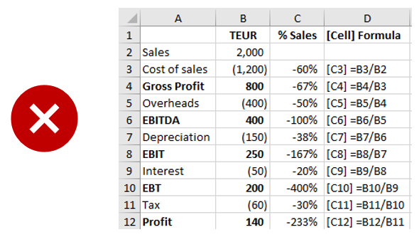
❌😣 A client wanted to calculate the percentage of sales for all P&L lines. Such a ‘common size P&L' is useful for comparisons e.g., of years or of different companies. His first formula in row 3 (see screenshot above) gave a correct result. But when he copied this down, the denominator in each formula referred to the row above and not the sales figure in row 2.
📗 This is because cell references in copied formulas are automatically amended by Excel e.g. to refer to cells in the same relative row or column. The technical term for this is relative referencing. Often this makes sense e.g. you want a copied SUM formula to always add up the values in the same column as the SUM formula. But sometimes (as in this example) this isn’t what you want.
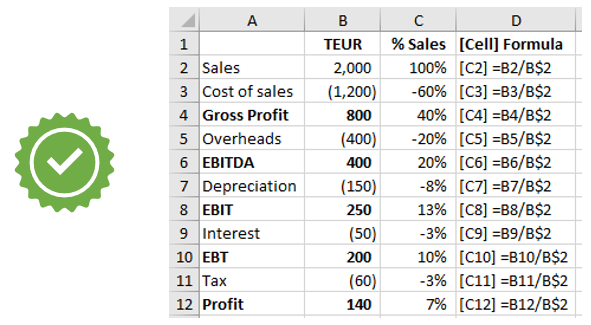
✔🤑 Here the denominator in the formula should always refer to the sales value in row 2 (cell B2), so the formula must read = (cell with value)/B$2. The dollar sign in front of the row number 2 fixes it, so it does not change when you copy the formula (see screenshot above).
💡 You can fix a column or row or both by manually typing in the dollar sign at the appropriate place(s) in your formula. Alternatively simply press F4 when the cursor is in or next to the relevant cell reference. This fixes (puts a dollar sign in front of) both row and column. Press F4 again to fix just the row. Press F4 again to fix just the column. Press F4 again to remove the fixing completely as the following example sequence shows.
B2 ➡ $B$2 ➡ B$2 ➡ $B2 ➡ B2
You can remember this order as follows: both, row, column, none. With practice, it becomes second nature to press F4 twice to fix the row only or three times to fix the column only.
As a general rule for fixing: Fix as much as necessary but as little as possible. In the example, it is only necessary to fix the row. And always review the results to identify and correct any errors.
This is just one of many how2excel tips you will find in my best practice book: Avoid Excel Horror Stories available on Amazon.