Gary’s Golden Ground Rules

😲 Nearly 90% of spreadsheets contain errors and many are also hard to use!
💰 These can be expensive in terms of money, time and reputation.

So how can you avoid these issues?

For my new book I went back to basics and completely overhauled my best practice advice. The result is my new, improved…

🥇 Gary’s Golden Ground Rules

These will help ensure that your spreadsheets are clear and easy to follow, which in turn reduces the risk of error during both development and usage.

1. Use a clear, logical workbook structure
Decide what worksheets you need, give them clear names and get them in order.

  • Spread content logically over worksheets
  • Organise worksheets into sections to reflect data flow from inputs to outputs
  • Include a cover sheet, ideally with hypertext links to facilitate navigation
  • Separate inputs, calculations and outputs


2. Keep your worksheets as clear and simple as possible
Ensure each worksheet is clearly laid out and easy to use.

  • Use a logical structure within each worksheet such as
  • Use consistent columns, row, formulas and whole sheets
  • Formulas
    • Ensure calculations flow from left to right and from top to bottom
    • Use the KISS principle: Keep It Short and Simple
    • Follow formula priorities: (i) correct, (ii) understandable and (iii) short
    • Follow the COUNT principle: Calculate Once, Use Numerous Times


3. Use a clear, clean, consistent design
Ensure the whole workbook has a clear, professional look and feel.

  • Use consistent (company-defined) fonts, colours, styles and data formats
  • Use the four key design principles: contrast, repetition, alignment and proximity
  • Clearly mark all inputs, for example as grey cells
  • Minimise non-data ink such as borders


4. Restrict access, inputs and changes
Ensure that only authorised users can access and change your spreadsheet and that inputs are valid.

  • Restrict access to the spreadsheet using folders with restricted access and passwords
  • Use data validation where relevant to help ensure inputs are valid - see my video for details
  • Consider protecting workbooks so that changes can only be made in input cells - see my blog for details


5. Write instructions for users
Ensure that users know what to do and in what order e.g., how to update the model with new data.

  • Create a worksheet with an action list for users to follow
  • Add a status column to ensure progress is clear


Interested to find out more? My book contains lots more details and plenty of examples and screenshots. Check it out on Amazon.

Do you COUNT?

COUNT stands for ‘Calculate Once, Use Numerous Times’. That means if you need to use a value multiple times, you should calculate it just the once and then link back to that value in all subsequent calculations. This can make your calculations shorter, easier to understand and faster.

Here you can see the logic. Using the COUNT method is simply more efficient.

Here are two examples to show how this works...

Example 1: Actual vs plan sales, month to date

In this example I want to compare the actual month-to-date sales with the planned month-to-date sales for each brand. For the planned sales I only have figures for the whole month and need to multiply these with the percentage of sales days so far (the month-to-date %).

  • COUNT method: The month-to-date % is the same for all brands so I calculate the figure once and use the result for each brand.
  • Non-COUNT method: I calculate the month-to-date % multiple times, once for each brand.


The COUNT method is more efficient than calculating the percentage again and again for each and every brand and it speeds up calculations. This is particularly important for large or complex spreadsheets that can take a while to calculate.

Example 2: Sales by year for a selected region

This example uses INDEX and MATCH. Here we want to retrieve the annual sales values for a selected region.

  • COUNT method: The data for the selected region is always in the same row, so I only need to calculate this row number once (with MATCH) for use in all INDEX formulas.
  • Non-COUNT method: The row number is calculated again and again, in each INDEX formula.


Using the COUNT method, the formulas are much shorter than the non-COUNT method, and so are easier to understand and also faster.

This is just one of the many tips I explain in my book Avoid Excel Horror Stories. Read more here or buy it on Amazon.

Knott Consulting Gary Knott - Buch How to Excel

Complete Excel tasks in a second

This is the final blog in a series of three to help you save time when working in Excel:

  1. Save time with the best Excel shortcuts
  2. Save time with the Quick Access Toolbar
  3. Complete Excel tasks in a second (this blog)

You can complete many common Excel tasks in a second!

I was inspired by this youtube video on how formula 1 pit stop times have been dramatically reduced and the accompanying LinkedIn post by Florian Palatini on the #SMED concept which covers 6 basic principles.

I have now adapted these principles to Excel… and speeded it up!

I call it #SSET = SINGLE SECOND EXECUTION OF TASK

🚀 Complete commonly performed Excel tasks in just a single second! 🚀

If you follow the advice in this blog, I estimate that you can easily save 10% of your time working in Excel. If you worked full-time in Excel, that would mean you would save four hours a week or 22 days a year!

Ready to learn?

On your marks, get SSET, go!

Read on or download the summary: Save hours of work in Excel.


1) Be prepared

Keyboard shortcuts: Learn your shortcuts - see my blog or download The Best Excel Shortcuts - a free list of the best Excel shortcuts to print out and refer to.

🖱 Quick Access Toolbar (QAT): For tasks where no shortcut is available, make sure you set up your QAT so that mouse-based tools and macros that you use regularly are lined up ready to use and always visible (no mouse clicks needed to show them!). In my blog I explain how.

Automation: For multi-step repetitive tasks, set-up Power Query, an office script or a macro to automate the actions. Store commonly-used macros in your personal workbook, so they are always available for use in any workbook and add those you often use to your QAT.

💥 Add-ins: Install one or more add-ins to add extra one-step buttons to further speed up your work. For a start, you can download my toolKCit add-in with 19 useful commands at eloquens for free.

Or check out these other add-ins:
https://www.ablebits.com/
https://www.arixcel.com/
https://www.martforexcel.com/
https://macabacus.com/
https://www.numeritas.co.uk/download-nxt/ - workbook auditing
https://www.operisanalysiskit.com/ - OAK tool for workbook auditing


2) Use precise locations

  • Desk - keep a clear desk with only the essentials on it, all suitably positioned.

  • Keyboard - ensure your keyboard is suitably placed in front of you so that you can easily use shortcuts.

  • 🖱 Mouse - ensure your mouse is suitably placed under your dominant hand to facilitate quick access to your Quick Access Toolbar (commonly used commands) and standard ribbon (infrequently used commands).


3) Follow a standard procedure

For each task that you commonly perform, decide what your ONE method is: select this based upon speed and convenience

  • Keyboard shortcut (if available) or
  • Quick Access Toolbar or
  • Automated solution - Power Query, office script or macro
  • Add-in


In this way, you also save thinking time, which speeds up your work some more.


4) Practise, practise, practise

As the building site worker said to the old lady who asked, “How do I get to Carnegie Hall?”
“Lady, you gotta practise!”

  • Use your keyboard shortcuts and your Quick Access Toolbar as often as possible to make their usage second nature.
  • Practice common tasks such as navigating, selecting, formatting, inserting, copy and pasting cells, rows and columns.


5) Adapt the equipment

Keyboard shortcuts: Learn new ones, as necessary.

🖱 Quick Access Toolbar: Amend as necessary to speed up your work. For example, add any missing but commonly used commands, remove any unused commands (to reduce clutter and make space for others) or move commands in the list so that they are in an order that you find logical and easy to locate.

Automation: Amend your Power Query, office scripts or macros, as necessary.

💥 Add-ins: Research, try out and install new add-ins.


6) Never stop looking for waste

Strive to learn new functionality and tricks and tips to save you time. Review tasks that you commonly perform but which take you time and try to identify improvements e.g., reduce the number of actions needed, use a new shortcut or a new button on your Quick Access Toolbar.


So now you know the secrets of how to complete Excel tasks in a second!

Put them into practice quickly!

Save time with the Quick Access Toolbar

This is the second blog in a series of three to help you save time when working in Excel:

  1. Save time with the best Excel shortcuts
  2. Save time with the Quick Access Toolbar (this blog)
  3. Complete Excel tasks in a second

What is the Quick Access Toolbar?

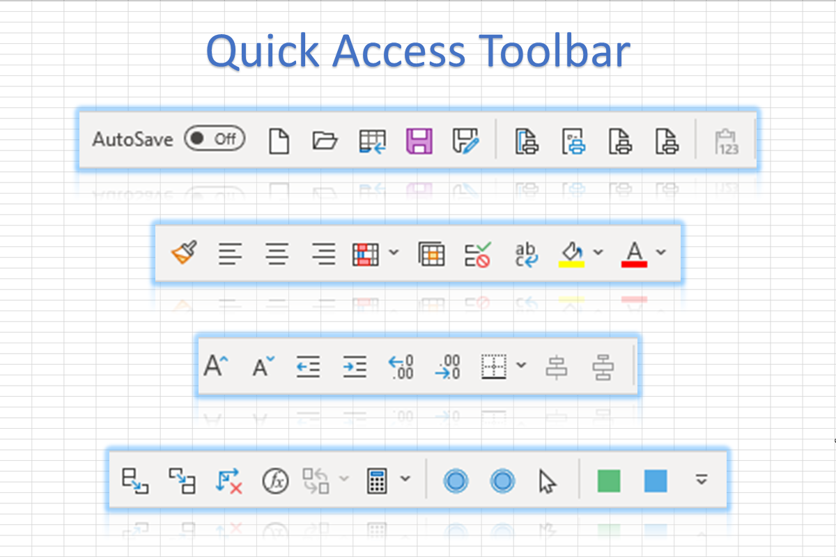
This is a narrow toolbar of small task icons which by default appears above the Excel ribbon and looks something like this.

These toolbar icons are always visible and so give you quick access to common tools - you don’t have to search through the detailed ribbons to find what you are after.

And the great news is, you can customise it yourself to contain tools which you regularly use, ready for quick access… hence the name: Quick Access Toolbar (QAT). These are then lined up ready to use and always visible - no mouse clicks needed to show them!


Where is it?

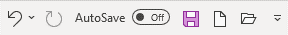
By default it sits above the menu and ribbons at the top of the Excel screen and contains just a few items like New, Open and Save.

I recommend that you use the option “Show Below the Ribbon” to reduce the amount you must move the mouse and to create more space for icons. Simply click on the down arrow at the far-right end of the QAT   and from the long list select  at the end.


How can I use it?

Use it exactly the same as the standard Excel ribbons. Click on an icon to carry out that command.


How can I customise it?

Start by clicking on the down arrow at the far-right end of the QAT and then you get a list of commonly-used tasks such as new, open, and save.

Those items in your QAT have a tick mark next to them. Simply click on relevant items to add them to or remove them from your QAT, as you see fit.

At the end of this list you will see the option “More commands”. Click on this to go into the detailed customisation and don't be shocked by what you see - it looks a bit complicated but is quite easy to use! I will show you how.


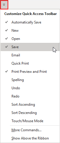
“Customise the Quick Access Toolbar” has four main sections, numbered in the screenshot above.

  1. Available commands: On the left you can select the commands that you want to add to your QAT. Find a command you want, click on it to select it. You can also select <separator> (first item in the list) which is a thin vertical line to optically separate sections of your QAT.

  2. Add/remove: Click the “Add >>” button to add the selected come and to your QAT on the right. The new items will be added below the QAT command that is currently selected in section 3.

  3. QAT: Here you can see the list of commands on your QAT. To remove a command, click on it to select it, then use the "<< Remove" button (in section 2, below the "Add >>" button).

  4. Up and down: To move a command in the QAT list, click on it to select it, then use the up and down arrow buttons to move it to your desired location.

When you are finished click OK to accept all the changes made.


How can I find a specific command?

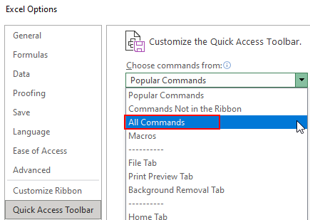
Everything in the ribbons and more(!) is available here. By default, the list shown in section one on the left contains only popular commands. Click on the down arrow to select other options for example “All Commands”.


 how2excel tips

Quickly add and remove QAT items:
To add: Simply right-click on an icon in an Excel ribbon and select "Add to Quick Access Toolbar".  It will be added at the end. To change the position, you need to us the more detailed customisation dialogue explained above, and the up and down arrows on the right.
To remove: Simply right-click on an icon in the QAT and select "Remove from Quick Access Toolbar".

Alternatively you can find and note down the names of the commands you want to add and then add these, as follows.

Find the name of a command: Commands are not always named the way you would expect. To find the name of the command which you are looking for, go back into normal Excel, find the command in the ribbon and hover over it. A tooltip appears, starting with the official name of the command - this is the name you need to search for in “Customise the Quick Access Toolbar”.

Find the command in the list: To avoid lots of scrolling, simply click somewhere in the list of command and type a letter e.g. D to jump to the first item starting with that letter.

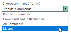
Add macros: To add a macro to the QAT, first select macros from the drop-down list in section 1.

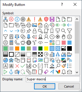
Then select and add your (macro) command as usual. Note that macros stored in your personal workbook start with the name personal. It makes sense to customise the appearance of macro items in the QAT. To do that, select the relevant (macro) command in the QAT (section 3), then click on the modify button at the bottom.

You can then select an appropriate icon and change the name which will be displayed when you hover over the icon in your QAT.


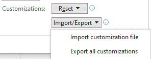
Export and import your customisations: After you have painstakingly customised your QAT, you may wish to make a back-up or give a copy to a colleague. Simply use the import/export button at the bottom on the right to export or import, as appropriate.


And action!

It can take a little while to get your QAT set up exactly the way you want it, but the investment of your time is well worth it. You then have very quick access to the commands and macros that you use a lot and this can speed up your work as you save you lots of time searching for items in the standard Excel ribbon.

Save time with the best Excel shortcuts

Gary Knott | how2excel - Excel Schulungen Downloads

This is the first blog in a series of three to help you save time when working in Excel:

  1. Save time with the best Excel shortcuts (this blog)
  2. Save time with the Quick Access Toolbar
  3. Complete Excel tasks in a second

You can get lots of things done quicker in Excel if you use keyboard shortcuts. Learn the best ones here.


What are the best Excel shortcuts?

I'm glad you asked! There are hundreds of shortcuts in total, but you can't learn them all, and many are for actions which you rarely perform. Therefore focus on the best ones.

Here is my list, organised by category to help you find the ones you need more easily. Read on or download a free one-pager to print out and use here: The Best Excel Shortcuts.


INPUT and EDIT

Key combination

Action

Description / comment

Ctrl Enter

Multiple input

Value or formula is input in all selected cells

Ctrl Shift ;

Input today's date


F2

Edit mode

Formula can be edited, precedents are marked in colour

F3

Call up range names

During the input of a formula, range names can be called up for selection

F4 (when entering or editing a formula)

Fix the row or column of a cell

Press repeatedly to cycle through the four variations: row and column with $ fixed, only row, only column, neither fixed


NAVIGATE

Key combination

Action

Description / comment

Ctrl Home

Go to home cell on sheet

Cell A1 or the first cell below frozen rows/columns

Ctrl End

Go to last cell on sheet

If there are many empty rows/columns above/left of this cell, delete these (after backing up your file) to reduce the file size

Ctrl Arrow (left, right,
up or down)

Go to end of row/column block


Ctrl Page up or down

Select sheet to the
left or right

Also works when you are writing a formula to select a cell on another sheet

Alt Page up or down

Show section to the
left or right

Also works when you are writing a formula to select a cell in another area

F5 or Ctrl G

GoTo cell or
special cells

1) Input cell reference and select "OK" or press Enter
2) Use "Special" to go to special cells

Ctrl Tab or
Ctrl Shift Tab

Go to next workbook

Also works when you are writing a formula to select a cell in another workbook


CALCULATE
(when calculation option is set to manual)

Key combination

Action

Description / comment

F2 then Enter

Calculate selected cell


Shift F9

Calculate sheet


F9

Calculate all open workbooks


COPY and PASTE, INSERT and DELETE

Key combination

Action

Description / comment

Ctrl C

Copy


Ctrl X

Cut


Ctrl V

Paste

After copying or cutting, can be used multiple times

Ctrl D

Copy down


Ctrl R

Copy to the right


Ctrl +

Insert cells, rows or columns

If appropriate, select row(s) or column(s) first

Ctrl -

Delete cells, rows or columns

If appropriate, select row(s) or column(s) first


FIND, SELECT and HIDE

Key combination

Action

Description / comment

Ctrl F

Find


Ctrl H

Replace


Ctrl A

Select block of data

Press Ctrl A again to select the whole worksheet

Shift Spacebar

Select row(s)


Ctrl Spacebar

Select column(s)


Ctrl Shift Arrow (left, right, up or down)

Go to end of row/ column block and select

Variations can be used one after the other, e.g. select to the left, then downwards

Ctrl 0 (zero)

Hide selected column


Ctrl 9

Hide selected row


FORMAT

Key combination

Action

Description / comment

Ctrl 1

Format cell(s)

Shows the format cells dialogue

Ctrl !

Format as value

With thousand markers and two decimal places

Ctrl $

Format as currency

With thousand markers and two decimal places

Ctrl %

Format as percent

With no decimal places

Ctrl &

Add outline


Ctrl #

Format as date

Month is shown as shortened word (Jan, Feb etc.)

Ctrl B

Format bold

Use key combination again to reverse the formatting

Ctrl I

Format italics

Use key combination again to reverse the formatting

Ctrl U

Underline

Use key combination again to reverse the formatting


OTHER

Key combination

Action

Description / comment

Ctrl P

Print

Works in all MS-Office applications

Ctrl S

Save file

Works in all MS-Office applications

Ctrl Z

Undo

Works in all MS-Office applications

F4 or Ctrl Y

Repeat

Repeats last action. Works in all MS-Office applications

Ctrl Shift `

View formulas

Use key combination again to return to normal view

F11 or Alt F1

Quick Chart

Select a block of numbers then use the shortcut --> a graph appears on a new sheet (F11) or on the same sheet (Alt F1)

Alt =

Auto sum

Creates a formula for the sum of the values above the cell (by default) or to the left of the cell (if there are no values above)


My favourite function is not listed - does it have a shortcut?

There is a simple way to find out… hover over an item on a ribbon until a tooltip with extra information appears. If there is a keyboard shortcut, Excel reveals what this is in brackets.

Shown above are two examples: Autosum (Alt =) and Show Formulas (Ctrl ´).

Confusingly Excel also shows you a plus sign which just means you must press the other keys at the same time, not that you must also press the + key.


No shortcut available or you are a mouse fan 🐭 ?

For tasks where no shortcut is available, or if you prefer to use the mouse, make sure you amend your Quick Access Toolbar so mouse-based tools that you use regularly are lined up ready to use and always visible (no mouse clicks needed to show them!)

My blog on the Quick Access Toolbar explains all you need to know.