Category: Blog EN

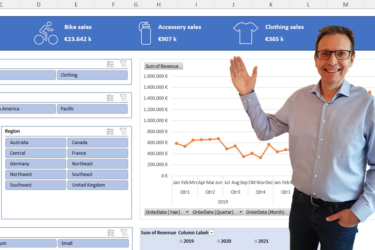
You can easily add icons, stickers, illustrations and more to your Excel file. You can use these to spice up your dashboards to show an icon next to key output figures such as “Bike sales”.

Simply follow the six simple steps shown in the screenshot.

1. Select Insert
2. Select Icons on the ribbon
3. Select Icons in the dialog box
4. Enter one or more search terms or select a category from those provided (not shown in the screenshot as they disappear as soon as you start to search)
5. Click on the icons you want
6. Click on “insert"

Each icon is generally available in two versions: unfilled (white) and filled (shown black).

Once inserted in your file, you can move them around and format them e.g. to change the colour. Select an icon and you get an extra ribbon "Graphics Format" with various options.

You can add a text box next to your icon with a description and another text box with a value. You can make this dynamic so that the value updates depending upon the current content shown on your dashboard: simply enter a formula for the text box in the formula bar = (cell with value). You cannot perform any calculations here (e.g. using IF), so perform these, if necessary, in the source cell.

Get more great tips by signing up for my Excel tips newsletter and also get access to free downloads.

Did you know? Excel now has a Quick Analysis tool.

⚡📈 Select some data and the Quick Analysis icon appears at the bottom right with lots of options organised in the following areas:

• Formatting
• Charts
• Totals
• Tables and
• Sparklines (mini charts in individual cells).
  
  

For example: If you have multiple columns to SUM, you can use the Quick Analysis tool like this.

1. Select your data
2. Select the Quick Analysis tool that appears (or use the shortcut Ctrl Q)
3. Select Totals
4. Select Sum

🤩 Check it out!

❌😣 A client wanted to calculate the percentage of sales for all P&L lines. Such a ‘common size P&L' is useful for comparisons e.g., of years or of different companies. His first formula in row 3 (see screenshot above) gave a correct result. But when he copied this down, the denominator in each formula referred to the row above and not the sales figure in row 2.

📗 This is because cell references in copied formulas are automatically amended by Excel e.g. to refer to cells in the same relative row or column. The technical term for this is relative referencing. Often this makes sense e.g. you want a copied SUM formula to always add up the values in the same column as the SUM formula. But sometimes (as in this example) this isn’t what you want.

✔🤑 Here the denominator in the formula should always refer to the sales value in row 2 (cell B2), so the formula must read = (cell with value)/B$2. The dollar sign in front of the row number 2 fixes it, so it does not change when you copy the formula (see screenshot above).

💡 You can fix a column or row or both by manually typing in the dollar sign at the appropriate place(s) in your formula. Alternatively simply press F4 when the cursor is in or next to the relevant cell reference. This fixes (puts a dollar sign in front of) both row and column. Press F4 again to fix just the row. Press F4 again to fix just the column. Press F4 again to remove the fixing completely as the following example sequence shows.

B2 ➡ $B$2 ➡ B$2 ➡ $B2 ➡ B2

You can remember this order as follows: both, row, column, none. With practice, it becomes second nature to press F4 twice to fix the row only or three times to fix the column only.

As a general rule for fixing: Fix as much as necessary but as little as possible. In the example, it is only necessary to fix the row. And always review the results to identify and correct any errors.

This is just one of many how2excel tips you will find in my best practice book: Avoid Excel Horror Stories available on Amazon.

You have customised a chart, then copied both chart and related data to another area ready for new data. You then amend the copied data, e.g. to show sales of a different business and…. oh! There is a problem…

What you expect

The copied chart should be linked to the copied data – this is logical but not what actually happens.

What you get

The copied chart is linked to the original data so doesn’t change when you amend the copied data. The selected data for the copied chart must be manually edited. This is a pain. ☹

And when you do that, you may well notice a second problem…

If you have edited the original chart e.g., changed line colours, added customised markers and data labels, these are mostly lost when you amend the data source in the copied chart. ☹

↪ The workaround

You can copy the entire sheet, then cut and paste the data and graph on the copied sheet back to the original sheet, but this is inefficient. You may also have to edit the axis labels e.g., for years if these were linked to a row at the top of your (copied) worksheet.

✔ The proper solution

Dear Excel development team at Microsoft… will you please fix this?

🗳 Your vote counts

Please like my related post on the official Excel community by clicking on the up arrow icon.

Calculation Options

If you have a large workbook with lots of lookup formulas or complex calculations the whole workbook can be slow to recalculate so you can turn on the manual calculation option.

There are two ways to do this:

1. File, Options, Formulas
   
   
   
2. Formulas ribbon, Calculation, Calculation Options (click the down arrow to open the dropdown)
   

In each case you will see three or four options:

• Automatic (standard setting) - generally recommended so that you can see the effects of spreadsheet changes immediately.
  
  
• Automatic except for data tables - recommended if you have data tables in your spreadsheet. Data tables are great for calculating the results of different scenarios to compare them but require multiple calculations of your model so this option is highly recommended in such cases to avoid slowing your model down unnecessarily.
  
  
• Manual - recommended for large and slow workbooks - this makes it much easier to work with your file but you can't see the effects of changes immediately, hence you need to manually initiate a recalculation (see below).
  
  
• Manual: Recalculate workbook before saving - this extra option is only available via File, Options. I recommend that you turn this off if you save your file often (e.g., so that in the case of a crash you have a recent copy of your file) but do not want Excel to recalculate your file each time as this can take a while with large, slow models.

Under File, Options you also get options for iterative calculations. This can be turned on if you have logical circular references on your model e.g., interest costs affect the closing bank balance which then affects the interest costs. The standard settings (100 iterations, maximum change 0.001) are generally good but, if necessary, you can increase the number of iterations and/or reduce the maximum change. Note that the accuracy here also appears to be used for Goal Seek calculations, so you can also make such changes to improve the accuracy of goal seek results.

 

Recalculation options and shortcuts

If you are using the manual calculation option, then you will have to manually start a recalculation at a suitable point in time (e.g. when you have completed a new model section). Here there are also a few options, some available with the ribbon/mouse, others with keyboard shortcuts as follows.

• Calculate now (shortcut F9) - recalculates all open workbooks. Close unnecessary files to speed this up.
  
  
• Calculate sheet (shortcut Shift F9) - recalculates only the currently active sheet. This is quicker than recalculating the whole workbook if you only need to update/check a single sheet.
  
  
• Calculate a single cell (shortcut only: F2 followed by the enter key) - recalculates only the selected cell. This is the quickest option, but only a single cell, useful on large sheets where even a calculate sheet takes a while. If you select a block of cells, you can press F2 and enter repeatedly to calculate each one in turn, Excel then jumps to the next cell.
  
  
• Force full recalculation (shortcut only: Ctrl Shift Alt F9) – this can be useful on the rare occasions when model results do not appear to reflect recent changes you have made. To reduce calculation time Excel normally only recalculates dependents of cells which have changed (and their dependents etc.) plus all volatile functions such as TODAY, INDIRECT and OFFSET. Normally this works very well. Very occasionally however, it can be useful to force a full recalculation. This can take a while, so close unnecessary files before you start.

 

toolKCit add-in tools

For ease of use and additional calculation options and tools you can buy and install my Excel add-in toolKCit, available for a small fee at eloquens. Use the discount code HOW2EXCEL for 50% off.

• Set manual calculation – sets the calculation to manual and no recalculate before saving. This is the same as going via File, Options but with a single mouse-click.
  
  
• Calculate with timer – performs a normal recalculation (like F9) but tells you how long it took. Useful when you are trying to speed up your model and wish to compare alternative calculations to see which is quicker.
  
  
• Force full recalculation – does the same as the shortcut mentioned above but with a mouse-click instead of the 4-key combination shortcut.