Category: Blog EN

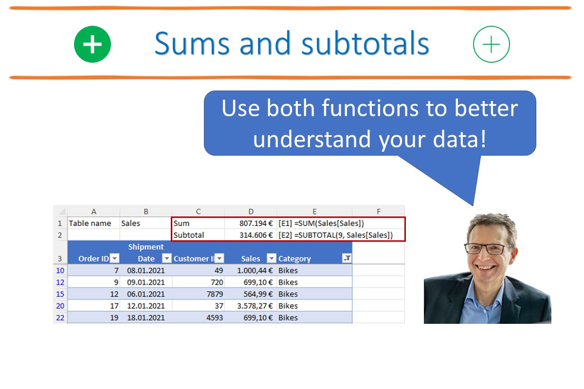
Use both SUMs and SUBTOTALs to help understand your data!

• Place SUMs for key data columns such as sales values above your data where you can easily see them and not below your data, which forces you to scroll down – that is inefficient, especially if you have long lists.
  
  
• Also calculate SUBTOTALs. SUBTOTAL is a very useful and flexible function which shows you the sum of your filtered data, very handy when checking or analysing your data.
  
  

The SUBTOTAL function can give various results depending upon the number you enter in brackets before the data range. Most commonly you want the sum, which requires the number 9. Other possibilities are average, count, maximum and minimum. As soon as you type SUBTOTAL( you get a drop-down list of all the options.

I recommend that you calculate both SUM and SUBTOTALS for key data columns in two separate rows, as shown in the screenshot. The SUM result showing the total of all amounts in the column is then always visible and can be linked onwards in the workbook (if necessary) and the SUBTOTAL can be used for filtering and data analysis. If no filters are set, the two formulas should give the same result.

Note: In the example in the screenshot I have used a table but both SUM and SUBTOTAL functions also work with data which is not in a table. In this case, simply enter the cell references as your data range.

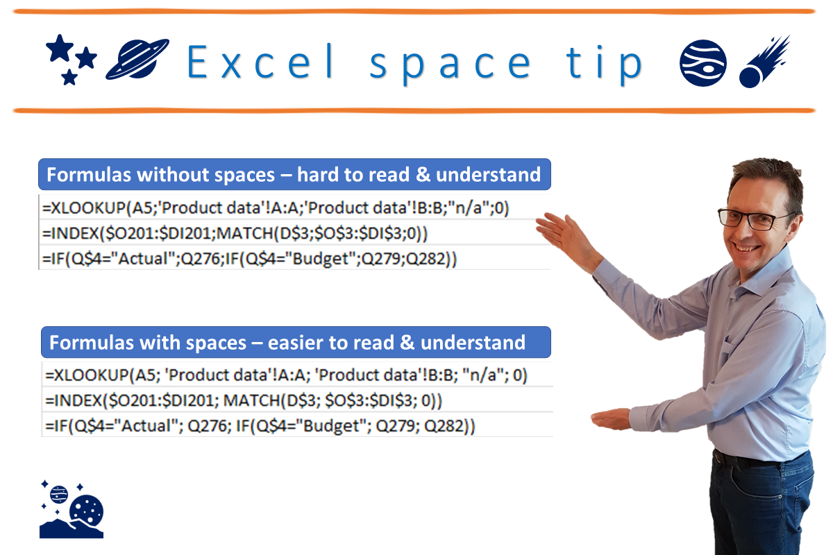
Did you know, you can add spaces to formulas to make them easier to read?

Well, you can, and you should! 😊

Inmedievaldaysbookswerewrittenbymonkswithoutspacesbetweenwords.

Did you find that easy to read? Of course, not – it has no spaces. But this was standard practice in medieval books. Over time, however, spaces were added between words to make texts easier to read.

When writing spreadsheet formulas, however, we are still mostly following the medieval monks. Surprise, surprise, this means that formulas – especially those which are longer or more complex – are harder to read. And harder to write, check, amend and understand.

Therefore, I recommend you add spaces to your formulas e.g., after every argument separator (a comma or semi-colon, depending on your regional settings) or before every plus-sign. This makes them easier to read etc. and has no impact on results as Excel ignores them.

Bonus tip: If you want to “retrofit” spaces into your formulas, make a back-up of your file then simply search and replace all argument separators (a comma or semi-colon) with a separator followed by a space.

We’ve all been there… a formula either isn’t accepted by Excel (syntax error), or it gives incorrect results (logic errors). Let’s look at these two cases in turn and see how you can best avoid or fix them.

1. Syntax errors

You finish typing in a formula, press enter, and Excel won’t accept it.

You get a hint such as “You’ve entered too few arguments for this function”. This may sound like Excel being fussy, but it really is quite helpful because you know what the error is, and this helps you find and fix it.

Here is a simple example using the function ROUND.

This simply means you were too quick to press the enter key. 😊

Watch the friendly tool tip which appears under the formula bar when you enter a valid function name followed by an open bracket.

Here Excel shows you exactly which argument you are currently entering by marking the name of the argument in bold. In this case, we have entered a cell reference referring to the cell containing the value that we wish to round and can see that we need a second argument called num_digits. If you are not sure what this means then you have two options.

• FX: Click on the “fx” icon in the formula bar and you open up the helpful “Function Arguments” dialog box which looks like this.

Here you can see the Num_digits argument and on the right-hand side it tells you it needs to be a number. Underneath you get a more detailed explanation. If this still is not enough then click on the link ”Help on this function” at the bottom to open up more details in a browser. These Microsoft help files contain explanations, helpful examples and often a video to help you understand.

• F1: Alternatively simply press F1 to call up the (shorter) help file within Excel.

If you know the function name and the arguments required you can type them in without paying attention to the helpful tooltip. But if you mistype a function name, you will get a #NAME error such as here where I have typed rund instead of round.

Simply retype your function name more slowly and Excel shows you a list of those functions containing the letters you have already typed for you to select the correct one with the correct spelling. It also gives you a helpful short explanation of what the first function does in a tooltip box.

To see what any of the other functions in the list do, simply move down the list with the down arrow on your keyboard or select one with your mouse.

Finally a word on optional arguments. If Excel shows you an argument in square brackets this means it is optional i.e. you don't need to enter anything and can simply close the brackets after you have entered the last compulsory argument (one not in square brackets). Here is an example with the MATCH function where the final argument match_type is optional.

This simply means it is technically optional, but an entry may be very necessary to ensure your function works as desired. In fact with the functions MATCH and VLOOKUP it is usually essential for correct functioning to enter a match type FALSE or 0 to ensure an exact match, otherwise Excel will simply look for the closest matching item, which may give you an incorrect result.

This brings us nicely to the second type of error which is harder to fix.

2. Logic errors

Here you have identified that although Excel has accepted your formula, it gives you an incorrect result.

The first step to solving this type of error is to use the F2 key to analyse the components of your formula.

In this example we can quickly identify that the formula refers to an incorrect cell.

In more complicated examples e.g. with nested IFs or AND conditions, it can be very helpful to click on a selected argument in the tooltip and Excel then marks the relevant section of your formula.

This can be helpful for identifying missing or misplaced brackets or separators (commas or, in this screenshot, semi-colons).

If that still doesn’t solve an issue, you can enlist the help of the Evaluate Formula tool on the Formulas ribbon.

This opens the evaluate formula dialogue box which shows you your formula and by clicking on the evaluate button at the bottom (or by pressing the enter key) Excel shows you how it evaluates the formula step by step so you can see exactly where you may be having a problem and correct the formula.

I hope these tips help to you to avoiding formula errors or, failing that, to detect and correct them.

For lots more tips on how to avoid detect and correct errors please refer to my book “Avoid Excel horror stories” available on Amazon.

STOCKHISTORY function

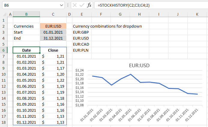
If you have Office 365 then you can use the function STOCKHISTORY. As the name implies, its main purpose is to enable you to retrieve stock prices, but it can also be used to retrieve historical exchange rates. This can be very useful e.g., for converting historical transactions to the reporting currency or assessing the volatility of foreign currency cash flows.

Exchange rates

In the screenshot you can see an example formula in cell B6. The arguments for the function (the bits inside the brackets) must include two ISO currency codes separated by a colon and a date range (dates from and to). Optionally you can specify the interval (0 = daily, 1 = weekly or 2 = annual) and whether you want opening or closing rates etc.

You only need to enter the formula once! It returns a dynamic array with column headers and as many rows of data as necessary. What is also great is that the values are so-called Formatted Number Values (“FNVs”) which means that Excel automatically formats the values with the correct currency symbol.

Stock prices and data type

You can, of course, also use this great function to get stock price values as the above screenshot showing historical Tesla stock prices demonstrates. The formula is basically the same but here the first input for the function is the stock ticker symbol, here TSLA for Tesla.

You can also define the cell with the ticker symbol as data type stock.

Now when you select the cell, you get an extra box with the option to add extra information such as price, 52 week high and 52 week low.

Data source

The source of all retrieved data is refinitiv, "an LSEG (London Stock Exchange Group) business, [and] one of the world’s largest providers of financial markets data and infrastructure."

More information

You can find out more about this function on the official Microsoft blog.

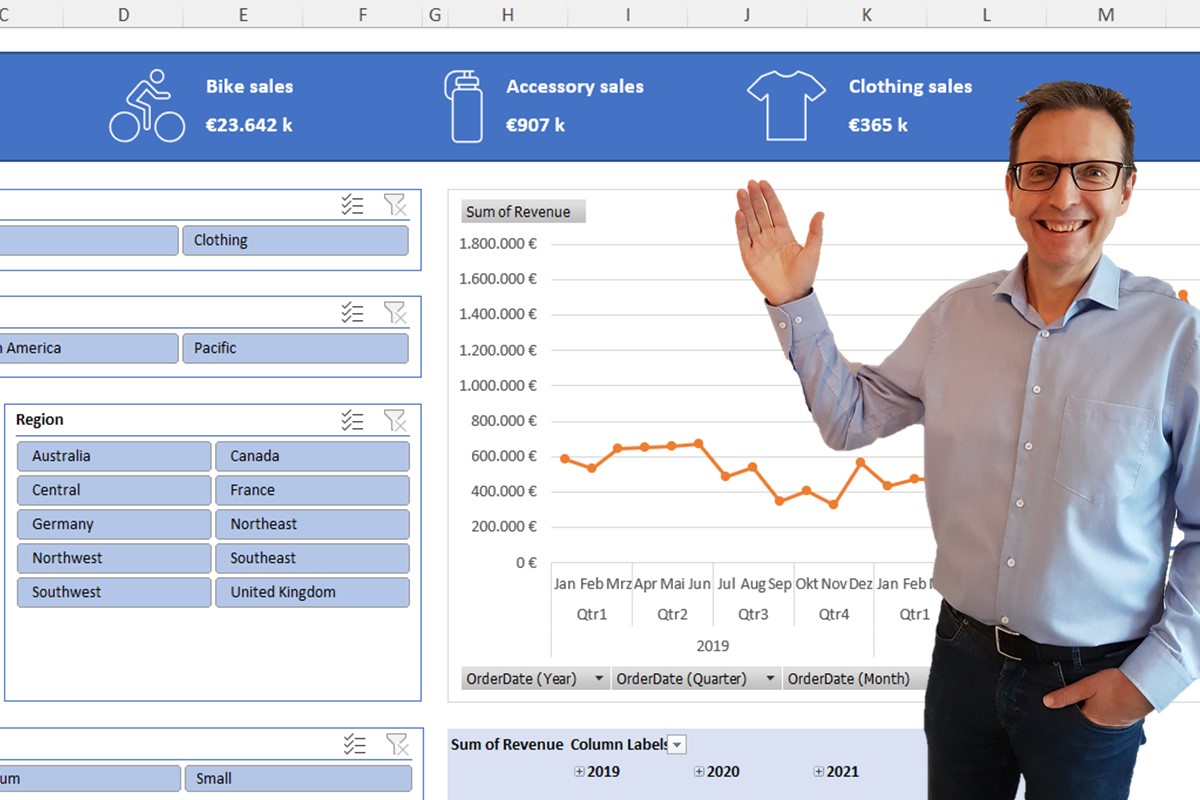
You can easily add icons, stickers, illustrations and more to your Excel file. You can use these to spice up your dashboards to show an icon next to key output figures such as “Bike sales”.

Simply follow the six simple steps shown in the screenshot.

1. Select Insert
2. Select Icons on the ribbon
3. Select Icons in the dialog box
4. Enter one or more search terms or select a category from those provided (not shown in the screenshot as they disappear as soon as you start to search)
5. Click on the icons you want
6. Click on “insert"

Each icon is generally available in two versions: unfilled (white) and filled (shown black).

Once inserted in your file, you can move them around and format them e.g. to change the colour. Select an icon and you get an extra ribbon "Graphics Format" with various options.

You can add a text box next to your icon with a description and another text box with a value. You can make this dynamic so that the value updates depending upon the current content shown on your dashboard: simply enter a formula for the text box in the formula bar = (cell with value). You cannot perform any calculations here (e.g. using IF), so perform these, if necessary, in the source cell.

Get more great tips by signing up for my Excel tips newsletter and also get access to free downloads.