Category: Blog EN

It's Christmas time again, the season of cheer. You can bring a little festive merriness to your PC by simulating Christmas advent candles using the magic of random numbers combined with conditional formatting.

Why not have a go yourself? I will show you how to develop two versions in just a few steps each. Alternatively you can download the finished version here: Christmas candles v3.

Basic version

Explanation: All four candles are always on.

Step 1 - Create your candles

Make columns narrow, then add background colours for the base, the candles and the wicks. Then add a message at the bottom plus festive icons and shapes (using the Insert ribbon), if you wish.

Step 2 - Add formulas

Enter these formulas in cells that should show flames:

=RANDBETWEEN(50, 100) for lighter flame colours
=RANDBETWEEN(1, 50) for darker flame colours in the centre, above the wick

These formulas generate random numbers every time a calculation is performed.  We will use these numbers to set the colours of the flames.

Step 3 – Add conditional formats

Select a block of cells containing the “flame cells” and add conditional formatting as follows.

Step 4 – Tidy up

For a cleaner look…

• Select then hide unused rows and columns (right click, hide)
• Remove the gridlines (View ribbon, Show section, deselect Gridlines box)
• Protect sheet (Review ribbon) and deselect all options to hide the cell selection
  
  

Step 5 - Animate

Press F9 to change the colours.  Or press and hold F9 to animate.

 

Advent Sunday version

Explanation: Each candle only lights up when the related advent Sunday is reached.

Step 1 – Create or copy the basic version

If necessary, unprotect the sheet (Review ribbon) and select and unhide all columns.

Step 2 – Add dates

• Today – enter formula =TODAY()
• Advent Sundays - input the four dates
  
  

Step 3 – Amend flame formulas

The formulas must now test if the relevant advent Sunday date has been reached. So each flame tests a different advent date, for example:

=IF($AR$10>=$AR$11; RANDBETWEEN(50;100); 0) for lighter flame colours in the first flame

If the relevant date has not been reached, the cell value is now set to zero.

Step 4 – Amend conditional formats

Add a second conditional format (tip: duplicate the first rule and amend it).

If the cell value is zero, format the colour to match the background so that no flame is visible.

Tidy up and animate

Same as the basic version.

 

Burning down candles version

In the the download file you will also find another version in which the candles gradually burn down!

I created this based upon (a copy of) the advent Sunday version and used the OFFSET function to simulate the burning-down based upon the number of days each candle has been burning and an input of how many days each row of candle picture lasts (e.g. 4 days), i.e. the "standard candle" offset by a number of rows.

Enjoy!

 

 

Here are two great ideas to create dynamic outputs e.g. for your dashboards: KPI cards and dynamic chart titles that automatically update when your data changes!

 

KPI CARD

A KPI card reports a single key value such as sales to date or a KPI - simple but great! They are common in Power BI, but you can also create them in plain old Excel. Here’s how.

• Insert a text box (Insert, Text box) or shape (Insert, Shape) - I like rounded rectangles – and format it as you wish.
• Select the shape and in the formula bar enter =(cell reference).
• If this is a number, the format in the text box or shape is the same as the source cell. 😊
• Extra tip: You can then add text around the number by double-clicking in the shape and typing!

 

CHART TITLE

Add a dynamic title to a chart e.g. with a date. Instead of accepting the default chart title or manually typing in your own title, you can link a chart title to a cell.

• Simply select the chart title box and in the formula bar enter =(cell reference).
• You cannot create a formula or use any functions here. But you can do that in the source cell…

• In the example shown, I want to include the latest date in the chart title. You can get this automatically using the function MAX on the date column in your source data or (as shown here) use an input cell (cell B25).
• I have created a dynamic title (in cell C25) using the date (in cell B25), which then appears in the chart title. Fantastic!
  • You can build this text in parts and join them using &
  • If you refer to a number or date, you must format this using the TEXT function.
  • To get the correct format, first select a cell with the format you want, go into format cell (shortcut Ctrl 1); on the “Number” tab, select “Custom”, then copy the ‘format code’ from the Type box.
    

• • Paste this into your TEXT formula inside quote marks.
  • In the example shown, the final formula is
    ="Sales month to date (EURk), as at " & TEXT(B25;"DD.MM.YYYY")
    
    
• Extra tip: You can hide your dynamic title cell behind the chart if you want to.

 

THE FINAL RESULT

Create range names

Select a cell or range of cells, then type in a short but descriptive range name in the Name Box (above cell A1, next to the Formula Bar) e.g., Start_date or Tax_rate. The name may not contain spaces (use an underscore if necessary) and certain names are not allowed e.g. J5 as this looks like a cell reference.

 

Use your range names

Here are three practical uses.

1. Simplify formulas

Simply start typing your range name in your formula and it will appear in the list along with function names (see screenshot above). Alternatively, press F3 to get a list to select from. This can make your formulas easier to read. In the example shown, a payment date cannot be in the past i.e. before the start date of the tool.

Karen Roem also likes the fact that the name does not change when you copy the formula, in contrast to a 'normal' link to a cell which you have to fix with dollar signs.

 

2. Easily select a range to copy

Here I have defined a range called AR which covers all the entries in the AR report. I can select this named range using the Name Box (above cell A1, next to the Formula Bar). I can then copy this (manually or using a macro) e.g. to another range AR_old, to allow comparisons to be made.

 

3. Aid navigation

(i) Use the Name Box

Simply use the Name Box dropdown (above cell A1, next to the Formula Bar)  and select a range name to jump to it.

(ii) Create a hyperlink

Alternatively, create a hyperlink using Insert, Link, Insert Link… (at the end of the list), Place in This Document, select a range name (under “defined names”) --> a clickable hyperlink is created in the cell. Simply click on it to jump to the range!

Bonus tip: You can copy this hyperlink to other places in your workbook if desired.

 

Edit and manage your range names

If you need to review or amend your ranges, simply use the Name Manager on the Formulas ribbon.

To reduce the risk of user error, you can protect your worksheets so that users can only change input cells and perform certain other restricted actions such as select cells and use filters. To enable this is a two-step process, as follows.

1. Ensure non-input cells are locked and input cells are unlocked

🔒 Non-input cells such as formulas and labels
By default, all cells have the status “locked” (protected). If you want to check, select all relevant cells, select Format Cells (shortcut Ctrl 1), select the “Protections” tab and check there is a tick next to the “Locked” property.

Hidden: The protection tab offers an additional option, ‘hidden’. This allows you to hide the cell formula in the formula bar when the cell is selected. In the interests of transparency and understanding a spreadsheet, I do not recommend this option.

🔓 Input cells
You must unlock the input cells (including those with data validation).

First, select the input cells. If you are not sure which cells are inputs, use GoTo (shortcut F5). Select “special” and “constants”, “numbers”, then ok. All input cells with content are now selected!

Then select Format Cells (shortcut Ctrl 1), select the “Protections” tab and remove the tick next to the “Locked” property.

Bonus tip #1: Use cell styles to easily remove protection for input cells

The easiest approach to unlock input cells is to use cell styles. Format an input cell with "Locked" turn off. Then go to the Home ribbon and click on the down arrow at the end of the the Styles section.

Select "New Cell Style..." and save the format as e.g. "01 Inputs" (numbering ensures your cell styles appear in your desired order).

Now when you want to format an input or drop-down cell in your model, simply select the cell(s) and click on the relevant style name in the styles box on the home ribbon. The cells are then given the appropriate colour and are automatically unlocked… simple and effective!

I typically use one cell style for inputs and another for drop-downs with a different colour, both of which are unlocked, i.e., the ‘locked’ option box is not ticked.

See Microsoft support for more details on cell styles.

Bonus tip #2: Use background error checking to identify missing protection

You can turn on background error checking for ‘Unlocked cells containing formulas’ under ‘File’, ‘Options’, ‘Formulas’, ‘Error checking rules’. Excel then automatically marks any unprotected cells with a green corner, and you can then correct the cell formatting, as explained above.

2. Turn protection on for each worksheet

This step is hinted at by Excel in the note underneath the protection settings. ‘Locking cells … has no effect until you protect the worksheet.’ This is simple enough to do.

🔐 Select the relevant worksheet, navigate to the Review ribbon, click ‘Protect Sheet’.

Then select what you want to allow. ‘Select locked cells’ and ‘select unlocked cells’ are allowed by default – generally sensible – but can be deselected. All other options are deselected by default but you can tick an option box in each case. One I generally allow is ‘Use AutoFilter’, especially for data analysis files or in models with large input sheets.

The final step is to input a password (if desired) and you are done. Obviously, you must remember the password, which can become a problem if you have lots of protected spreadsheets in use. You can therefore consider protecting the worksheet without a password to avoid problems.

Repeat for all further sheets in the model that you wish to protect. If you use a password, I strongly recommend using the same password for all protected worksheets in a single workbook otherwise the pain of password management or the risk of forgetting a password becomes too great.

🔓🔐 If you remove worksheet protection to make a change, you must re-protect it afterwards!

I am afraid there is no option to turn the protection on (or off) for all worksheets at once, so this task quickly becomes time-consuming, unless you use a macro…

Macro to the rescue!

I use a macro to protect all worksheets in a workbook and another to unprotect them all. To get this, please download my free bonus material for my book "Avoid Excel Horror Stories". The VBA macro code is in the main file ‘how2excel – example calculations and macros’.

The ‘protect sheets’ macro also solves another problem with protected sheets: by default, you cannot open and close row and column groupings on protected sheets (an Excel bug), which can be frustrating. As well as protecting sheets, the macro provided specifically enables the opening and closing of row and column groupings.

Bonus tip: Add password protection to the macros to prevent unauthorized users finding the password in the macro code! In Visual Basic editor, right-click macros, select VBAProject Properties, Protection tab, Lock project for viewing, enter password twice.

Extra protection: workbook structure

On the Review tab next to ‘Protect Sheet’ there is an icon for ‘Protect Workbook’. This enables you to prevent users changing the structure of a spreadsheet (e.g., moving, renaming, deleting or adding worksheets), which may be worth considering.

RESULT

In the suitably protected worksheet shown above, users can only enter and change values in the grey input cells. If they try to change any other cells, they get an error message like this.

Profit percent, percentage changes and average prices – all three are very useful for business but for each one there are two calculation methods so there is a risk of confusion and error.

In this blog I go through all three and in each case I explain the two calculation methods and recommend which one to use.

Let’s go…

 

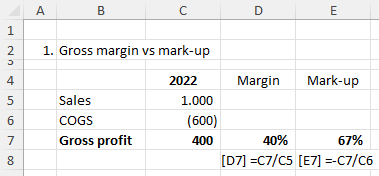
1. Gross margin % or mark-up % ?

Both of these figures are related to the gross profit, but they serve different purposes and are calculated differently.

Gross margin %

• Margin tells you what proportion of your sales is left as gross profit.
• It is useful for comparisons e.g., of two different products, two business units, two businesses, two years, or plan and actual figures. It can also tell you how much you can reduce selling prices by and still make a gross profit.
• The calculation is gross profit / sales.
• In the example shown above this is 400 / 1000 = 40%.
  That means that for every 100 Euros of sales, you are left with 40 Euros of profit (i.e. 40%).

Mark-up %

• Mark-up on the other hand tells you how much you add to your cost of goods sold (COGS) – i.e. what it costs you to buy or produce the products or services you are selling – to get your selling price.
• It is useful for calculating or assessing selling prices and is typically applied to individual products or groups of products.
• The calculation is gross profit / COGS; if your COGS figure is shown as a negative number, you can add a minus sign to your calculation so that the result is a positive number.
• In the example shown above this is 400 / 600 = 67%.
  That means that for every 100 Euros of costs, you add 67 Euros on top to get your sales price. For 600 Euros of costs you would add 600 * 67% = 400 Euros, which represents your gross profit.

Recommendation

In general, I recommend the margin %. Sales prices are often set in comparison to competitors (market-based pricing) or what you believe the value to be for your customers (value-based pricing). The concept of mark-up is then not relevant, but of course, you should still consider your costs.

The margin % is also consistent with a “single size profit and loss account (P&L)” analysis where all P&L items are calculated as a percentage of sales. This extends the approach for comparing e.g. two years or two businesses from comparing just the gross profit to comparing all P&L lines.

 

2. Change in percentage points or percent?

A change in percent is often used to plan or assess e.g. costs. If you are analysing monetary values, there is usually no confusion. If costs have risen form 1,000 Euro to 1,200 Euros then we have a 20% increase = 200 Euros rise / 1,000 Euros.

Things can get confusing however when you compare the change in a percentage figure, such as (i) cost of goods sold (COGS) as a percentage of sales or (ii) interest rates, as shown in the example below. Here the interest rate has risen from 10% p.a. to 12% p.a. (unrealistic but simple figures for the purpose of illustration).

Note: I took this example from the website https://www.mathsisfun.com, so thanks to them!

Here we can calculate and talk about the change either in percentage points or in percent and we must be clear which one we are using.

Change in percentage points

• The interest rate has risen from 10% to 12% so the change is simply 12% - 10% = 2% i.e. 2 percentage points and not 2 percent.

Change in percent

• The change in percent however is 20%, because the rise of 2% points is on top of the old rate of 10% = 2% / 10% = 20%.
• If we examine the interest costs, these have risen from 1,000 Euros p.a. to 1,200 Euros so we also have a 20% increase = 200 Euros rise / 1,000 Euros.

Recommendation

Both figures are correct, but you must be clear about which one you are using. In general, we are interested in the impact in monetary terms, which the change in percent figure tells us.

As the mathisfun website says, “When in doubt, use both. For example, say 'Interest rates increased by 2 percentage points today, meaning a 20% increase in interest payments.'"

 

3. Simple or weighted average?

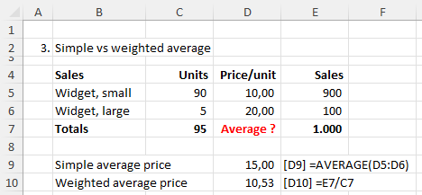
In this final example we are selling two products: a small widget and a large widget. The small version sells for 10 Euros each and the large version for 20 Euros each. What is the average selling price?

Simple average

• If you have no information on numbers of units sold (or you choose to ignore them), then you can calculate the simple average = (10 + 20) / 2 = 15 Euros
• This is really only true if you sell the same number of units of each product, which is probably not the case.
• In most cases, the simple average gives an incorrect understanding of the average price as we have not considered the numbers of units of each product sold. When we take these into account, this can have a dramatic impact on the average, as we will now see.
  
  

Weighted average

• The correct way to calculate the average selling price is to take the total sales divided by the total number of units sold.
• In this case we have 1,000 Euros total sales divided by 95 total units sold which gives a weighted average selling price of 10.53 Euros.
• This figure is much lower than the simple average of 15 Euros because it has been weighted by the number of units sold: we have sold many more units of small widgets than large widgets, so the weighted average price gets weighted towards the small widget price of 10 Euros.
  
  

Recommendation

Use the weighted average. To calculate this, you need to use total figures, as shown in the example above.

If you don’t have enough data to calculate the weighted average, state that the figure you show is a simple average. And don’t use it for calculations.